A pathway to more efficient generative models | Will Grathwohl | 2018 Summer Intern Open House

Invertible generative models can become more expressive and potentially more efficient by switching from discrete “flow steps” to a continuous-time formulation that replaces Jacobian log-determinants with an integral of divergence. In standard normalizing flows, each transformation must be invertible and the model must compute the log determinant of the Jacobian at every step—requirements that push architectures toward simpler, computationally friendly transformations. That simplicity forces models to stack many steps (as in Glow) to gain expressiveness, which can increase parameter count and compute.

A continuous normalizing flow reframes the model as parameterizing a dynamical system. Instead of applying a sequence of discrete transformations from time 0 to a final time, the model treats the data as evolving under a learned vector field. The likelihood then follows from the change-of-variables formula: in the continuous limit, the sum of log determinants becomes an integral over time of the divergence of the vector field. This shift matters because computing log determinants of arbitrary Jacobians is expensive—typically scaling like n cubed after forming the Jacobian—and there is no efficient unbiased estimator in general. Divergence, by contrast, admits an efficient unbiased estimator using automatic differentiation: sample a Gaussian “probe” vector, use it to probe the Jacobian via automatic differentiation (effectively estimating the trace of the Jacobian), and the expectation recovers the divergence. That estimator can be plugged into the continuous likelihood calculation to yield an unbiased estimate of log-likelihood, enabling training with standard backpropagation tools.

The tradeoff is computational. Discrete flows apply a known sequence of transformations; continuous flows require numerically integrating an ordinary differential equation (ODE) to transform samples and to evaluate likelihood terms. Training becomes harder because gradients must backpropagate through the ODE solution. Work from the University of Toronto provides a method to compute the needed gradients by solving an augmented ODE system, leveraging decades of numerical methods for ODEs to make the approach tractable.

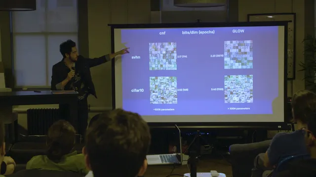
Empirically, continuous normalizing flows have been compared against Glow and RealNVP. The results reported are competitive with RealNVP, and in some datasets continuous normalizing flows even outperform Glow, though they have not fully beaten Glow yet. The main bottleneck is training time: continuous models currently take too long to train, limiting how large they can be made. A visualization example shows a learned gradient field warping digit images through time toward a Gaussian-like distribution; after integrating forward, the model can integrate backward to generate samples. The architecture described uses a single neural network that, at each time step, takes in the current image and the time value to parameterize the vector field, with the ODE integration performing the actual invertible transformation.

Overall, the approach offers a clear path to more flexible invertible generative models: use divergence-based likelihood estimation to avoid Jacobian log-determinant bottlenecks, then rely on ODE solvers and augmented-system gradient methods to keep training feasible. Remaining issues center on making training fast enough to scale model capacity and close the gap with the strongest discrete-flow baselines.