A quick trick for computing eigenvalues | Chapter 15, Essence of linear algebra

For 2×2 matrices, eigenvalues can be computed almost instantly by reading two numbers off the matrix—its trace and determinant—then using a “mean–product” version of the quadratic formula. The payoff is speed and, more importantly, a clearer mental model: the trace gives the sum (and thus the mean) of the eigenvalues, while the determinant gives their product. Once those are known, the eigenvalues must sit symmetrically around the mean, so the remaining work reduces to a single square root.

The standard route starts from the eigenvalue condition: if λ is an eigenvalue of a matrix A, then A − λI sends a nonzero vector to zero, forcing det(A − λI)=0. For 2×2 matrices, that determinant becomes a quadratic characteristic polynomial, whose roots are the eigenvalues. Solving it typically means expanding, simplifying, and then applying the quadratic formula—work that’s not terrible, but it’s avoidable.

The shortcut relies on three facts, of which the first two are especially quick to extract from the matrix. First, the trace (sum of the diagonal entries) equals the sum of the eigenvalues. Equivalently, the mean of the two eigenvalues equals the mean of the two diagonal entries. Second, the determinant equals the product of the eigenvalues. For a concrete example, a matrix with diagonal entries 8 and 6 has eigenvalue mean 7, and if its determinant is 40, then the eigenvalues multiply to 40.

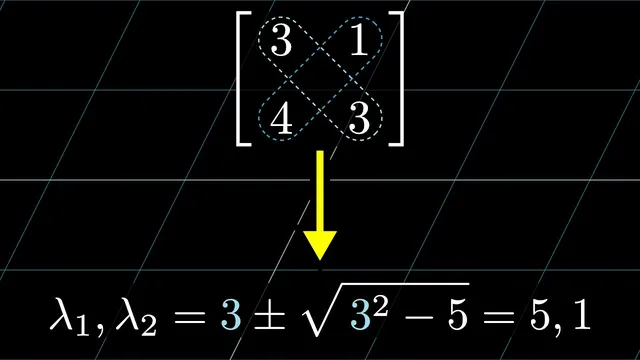
The third fact turns those two pieces into the actual eigenvalues. If two numbers have mean m and product p, they must be m ± d for some distance d. Their product becomes (m+d)(m−d)=m²−d², so d²=m²−p. That yields the general formula: the eigenvalues are m ± √(m²−p). This is essentially the difference-of-squares identity repackaged for eigenvalue problems, and it can be re-derived quickly if forgotten.

The method is demonstrated on specific 2×2 matrices where the trace and determinant immediately produce the eigenvalues with minimal algebra. It’s also connected to physics through the Pauli spin matrices, which have eigenvalues ±1. In that quantum-mechanics setting, the eigenvalues correspond to the discrete outcomes of spin measurements along chosen axes.

A key nuance: for those particular Pauli matrices, the traditional characteristic-polynomial method can be just as fast or faster. The real advantage appears when forming linear combinations of them—matrices built from a, b, c coefficients representing a direction in space. In that more general case, the trace remains easy to read (often still 0), and the determinant can still be checked quickly; then the mean–product formula pins down the eigenvalues without the heavier characteristic-polynomial expansion.

Finally, the shortcut is framed as a meaningful, not merely memorized, quadratic-solver: it mirrors how quadratic roots are determined by sum and product. The broader lesson is that trace and determinant aren’t just bookkeeping—they directly encode eigenvalue information, letting students skip the intermediate characteristic polynomial and write the roots straight from the matrix.