Abstract Linear Algebra 1 | Vector Space

Abstract linear algebra starts by stripping vectors of their familiar coordinates and rebuilding them from rules. The core move is defining a vector space as a nonempty set V equipped with two abstract operations: vector addition (taking two vectors in V and returning another vector in V) and scalar multiplication (taking a scalar from a field F and a vector in V, again returning a vector in V). This framework matters because it lets linear algebra work in settings far beyond R^n and C^n—any time objects obey the same algebraic laws, the same geometric and computational ideas can follow.

Once the two operations are in place, the definition becomes precise through a set of eight axioms. First, the vectors under addition must form an abelian group: addition is associative, there is a zero vector that leaves any vector unchanged when added, every vector has an additive inverse (so v + (−v) equals the zero vector), and addition is commutative. These properties ensure that vector addition behaves predictably even when vectors are abstract objects rather than arrows in space.

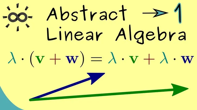
Next come the axioms tying scalar multiplication to the field F and to vector addition. Scalar multiplication must be compatible with multiplication in the field: scaling a vector by two scalars in succession must match scaling by their product in F. It also must respect the multiplicative identity of the field: scaling by 1 leaves vectors unchanged. Finally, two distributive laws connect scalar multiplication with addition. One law says scaling the sum of two vectors equals the sum of the individually scaled vectors. The other says scaling by the sum of two scalars equals adding the two separately scaled vectors. Together, these distributive rules guarantee that the “two different plus signs” (addition in V versus addition in F) interact correctly.

With these axioms satisfied, V becomes an F-vector space, meaning the choice of field is part of the structure. Real and complex vector spaces are highlighted as the most important cases, but the definition allows any field depending on the problem at hand. The practical takeaway is that computations and reasoning can be carried out inside this abstract setting much like in R^n and C^n. Arrow diagrams remain a helpful visualization, but the elements of V are not inherently arrows—those are just a mental model. The payoff is that later topics like linear maps, change of basis, inner products (for angles and orthogonality), and eigenvalues can be generalized to these abstract spaces once the vector-space foundation is secure.