Abstract Linear Algebra 2 | Examples of Abstract Vector Spaces

Vector spaces don’t have to be made of arrows or coordinates—once addition and scalar multiplication obey the usual rules, almost any structured collection of objects can qualify. The core takeaway is that sets of matrices, functions, and polynomials become vector spaces as soon as their natural operations (entrywise addition and scaling for matrices; pointwise addition and scaling for functions; coefficient-based addition and scaling for polynomials) satisfy the vector space axioms over an appropriate field like ℝ, ℂ, or even ℚ.

A first, familiar example is the set of all M×N matrices whose entries lie in ℂ, written as ℂ^{M×N}. Adding two such matrices is done entry by entry, and multiplying a matrix by a complex scalar scales every entry. Because these operations follow the standard algebra of complex numbers, the vector space axioms reduce to checking familiar properties like associativity, distributivity, and existence of additive identity and inverses.

The more conceptual example is a function space. Fix any set I and consider all maps from I to ℝ, denoted CurvF(I) (written as F^I in the transcript). This collection becomes a real vector space when addition and scalar multiplication are defined pointwise: for functions f and g, the sum (f+g)(x) equals f(x)+g(x) using ordinary addition in ℝ; for a real scalar Λ, the scaled function (Λ·f)(x) equals Λ·f(x) using ordinary multiplication in ℝ. The vector space axioms then “inherit” from the corresponding rules in the real numbers, since every required identity is verified by applying it at each point x∈I.

The same construction works for complex-valued functions, producing a complex vector space when scaling uses complex numbers.

A second major example is the space of polynomials. Let CurvP(ℝ) be the set of polynomial functions P:ℝ→ℝ, where P(x) is built from natural powers of x with real coefficients (P(x)=a_n x^n+…+a_1 x+a_0). Addition and scalar multiplication are defined using the same pointwise/coefficients-based operations as for functions, but with an important constraint: the result must still be a polynomial. That closure holds—adding two polynomials yields another polynomial, and scaling a polynomial by a scalar keeps it polynomial—so CurvP(ℝ) forms a real vector space. With complex scalars, it similarly becomes a complex vector space.

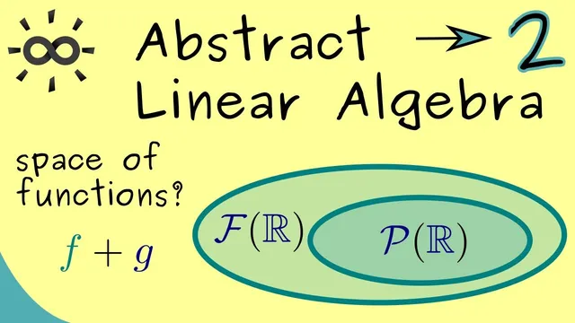
Finally, the transcript connects these examples by viewing polynomials as a subspace. Since every polynomial is a function, CurvP(ℝ) sits inside the larger function space CurvF(ℝ) (the set of all functions ℝ→ℝ). Because the vector space operations are the same, this inclusion is a linear subspace: it shares the same zero vector as the ambient space. In the function setting, the zero vector is the zero function—mapping every input x to 0—so the “abstract zero” in CurvP(ℝ) is exactly that polynomial/function.