Abstract Linear Algebra 26 | Matrix Representations for Compositions

TL;DR

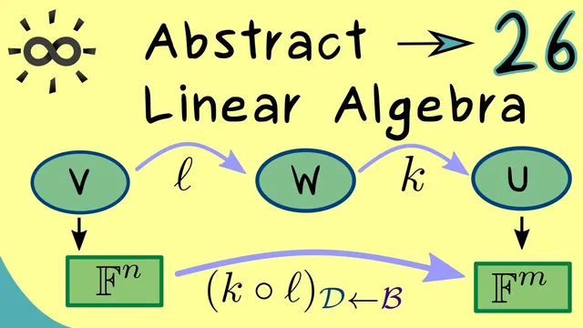
For linear maps L: V→W and K: W→U, the coordinate matrix of K∘L is the product [K]_{C→D} · [L]_{B→C} once bases B, C, and D are fixed.

Briefing Cornell Notes

Briefing

Matrix representations of composed linear maps follow the same rule as ordinary matrix multiplication: the matrix for K∘L is obtained by multiplying the matrix for K by the matrix for L, with the “middle” basis matching in the product. Concretely, if L: V→W and K: W→U, then choosing bases B (for V), C (for W), and D (for U) yields a matrix for L (size m×n) and a matrix for K (size k×m). The matrix for the composition K∘L (from V to U) is then the product [K]_{C→D} · [L]_{B→C}. This matters because it turns an abstract composition of linear maps into a concrete computation on coordinates—no need to re-derive the composition from scratch each time.

The transcript emphasizes how basis choices control the calculation. The “middle” basis C must be the one used to translate outputs of L into coordinates that K can consume. If the goal is the matrix of K∘L, picking a convenient basis for W can simplify both component computations and the final multiplication.

An example makes the rule operational. First, a linear map L sends vectors in R^3 to polynomials in P_2 using monomials m0, m1, m2 (with m0, m1, m2 corresponding to 1, X, X^2). The map is defined by sending (v1, v2, v3) to the polynomial with coefficients (v1+v2+v3) for m0, (v1+v2) for m1, and v1 for m2. With standard bases in R^3 and R^2, and choosing the monomial basis in P_2 as the intermediate basis, the matrix of L becomes a 3×3 matrix whose columns are the images of the standard basis vectors of R^3 expressed in the monomial basis.

Next, K maps P_2 to R^2 by using derivatives evaluated at 1. For a polynomial P, the first component is P′(1). The second component is P(1) minus P″(1). To build the matrix of K, each monomial m0, m1, m2 is fed into these derivative-and-evaluation rules. Constants differentiate to zero, X differentiates to 1 at x=1, and X^2 differentiates to 2 at x=1; similarly, the second derivative of X^2 is 2, which produces the needed entries in the second component. This yields a 2×3 matrix for K.

Finally, the composition matrix for K∘L is computed by multiplying the 2×3 matrix for K by the 3×3 matrix for L, producing a 2×3 matrix. The key takeaway is that the composition calculation can be performed entirely at the matrix level once the basis conventions are set.

The transcript closes by connecting this composition rule to invertibility. If L is invertible, then L^{-1} is also linear, and its matrix representation (with bases swapped) is the inverse of the matrix representing L. As a result, an invertible linear map corresponds to an invertible square matrix (determinant nonzero). This only works when domain and codomain dimensions match (n=m); if dimensions differ, a linear map cannot be invertible because its matrix representation cannot be square.

Cornell Notes

Composing linear maps becomes matrix multiplication once bases are fixed. For L: V→W and K: W→U, choosing bases B (V), C (W), and D (U) gives [K∘L]_{B→D} = [K]_{C→D} · [L]_{B→C}. The “middle” basis C is essential because it matches the coordinates produced by L with the coordinates consumed by K. In the worked example, L maps R^3 to P_2 using monomials {m0,m1,m2}, while K maps P_2 to R^2 using derivatives evaluated at x=1; the final matrix for K∘L comes from multiplying the two coordinate matrices. Invertible linear maps correspond to invertible (square) matrices, and L^{-1} is represented by the matrix inverse of [L].

Why does the matrix for a composition K∘L equal a product of two matrices, and where does the “middle” basis fit?

Because coordinates must be translated consistently between spaces. With L: V→W and K: W→U, pick bases B for V, C for W, and D for U. The matrix [L]_{B→C} converts B-coordinates in V into C-coordinates in W. Then [K]_{C→D} converts those C-coordinates into D-coordinates in U. Multiplying them aligns the output basis of L (C) with the input basis of K (also C): [K∘L]_{B→D} = [K]_{C→D} · [L]_{B→C}.

How is the matrix of L constructed in the example mapping R^3 to P_2?

L is defined by how it transforms a vector (v1,v2,v3) into a polynomial in P_2 with coefficients on the monomials m0,m1,m2. Using the monomial basis {m0,m1,m2} as the intermediate basis C, the columns of [L]_{B→C} come from applying L to each standard basis vector of R^3: B1=(1,0,0), B2=(0,1,0), B3=(0,0,1). Each image is then expressed as a linear combination of m0,m1,m2, producing a 3×3 matrix.

What is the practical method for building the matrix of K: P_2→R^2 in the example?

K is defined using derivatives evaluated at x=1: for a polynomial P, the first component is P′(1), and the second component is P(1) − P″(1). To form [K]_{C→D}, feed each monomial m0,m1,m2 into these formulas. Since m0 is constant, its derivative terms vanish; for m1=X, P′(1)=1 and P″(1)=0; for m2=X^2, P′(1)=2 and P″(1)=2. These computed two-component outputs become the columns of a 2×3 matrix.

How does the final matrix for K∘L arise from the example’s two matrices?

Once [L]_{B→C} is a 3×3 matrix and [K]_{C→D} is a 2×3 matrix, the composition matrix [K∘L]_{B→D} is obtained by one matrix product: [K]_{C→D} · [L]_{B→C}. The multiplication combines the columns of [L] (expressed in the monomial basis) with the derivative/evaluation action encoded in [K]. The result is a 2×3 matrix mapping R^3 coordinates directly to R^2 coordinates.

What condition makes a linear map invertible in terms of its matrix representation?

Invertibility requires a square matrix representation. If L: V→W is invertible, then dim(V)=dim(W), so the matrix of L is n×n (square). In that case, the matrix of L^{-1} is the inverse matrix of [L], meaning det([L])≠0. If dim(V)≠dim(W), the matrix is not square, so a linear map cannot be invertible.

Review Questions

Given L: V→W and K: W→U with chosen bases B, C, D, write the exact matrix formula for [K∘L]_{B→D} and explain why C appears in both factors.
In the example, compute the column of [K] corresponding to the monomial m2=X^2 using the rules P′(1) and P(1)−P″(1).
Why does invertibility of a linear map require dim(V)=dim(W), and how does that translate to the shape of its matrix?

Key Points

1
For linear maps L: V→W and K: W→U, the coordinate matrix of K∘L is the product [K]_{C→D} · [L]_{B→C} once bases B, C, and D are fixed.
2
The intermediate basis C is not optional: it must match the basis used to express L’s outputs so K can act on the same coordinate system.
3
Choosing a convenient basis for the intermediate space W can simplify both matrix construction and the final multiplication.
4
In the worked example, L: R^3→P_2 is built by taking images of standard basis vectors and expressing them in the monomial basis {m0,m1,m2}.
5
In the worked example, K: P_2→R^2 is built by evaluating P′(1) and P(1)−P″(1) on each monomial, producing the columns of a 2×3 matrix.
6
The matrix for an inverse map L^{-1} is the inverse of the matrix for L (with bases swapped), provided L is invertible.
7
A linear map can only be invertible when domain and codomain dimensions match, ensuring the matrix representation is square (n=m).

Highlights

Matrix representations of compositions follow the same rule as matrix multiplication: [K∘L] = [K]·[L], with the shared middle basis aligning the product.

The “middle” basis choice can turn a messy composition into straightforward coordinate calculations.

Using derivatives evaluated at a point (x=1) turns a polynomial-to-vector map into a simple column-by-column matrix construction.

Invertible linear maps correspond exactly to invertible square matrices, with L^{-1} represented by the matrix inverse of [L].

Topics

Matrix Multiplication
Linear Map Composition
Basis Representations
Polynomial Derivatives
Invertible Linear Maps