Abstract Linear Algebra 31 | Solutions for Linear Equations

Solving a linear equation in an abstract setting boils down to two geometric objects: the range (for whether solutions exist) and the kernel (for whether solutions are unique). For a linear map L: V → W between vector spaces over a field F (real or complex), the equation L(X) = B asks for all X ∈ V that land on a fixed target vector B ∈ W. Existence is immediate: if B is not in the range of L, there are no solutions. Uniqueness is equally tied to structure: if the kernel of L contains anything beyond the zero vector, then multiple solutions appear because different kernel elements can be added without changing the output.

In this framework, the kernel is defined as ker(L) = {v ∈ V : L(v) = 0}, meaning it is exactly the solution set of the homogeneous equation L(X) = 0. The range is defined as range(L) = {w ∈ W : ∃x ∈ V with L(x) = w}, i.e., the set of all right-hand sides that the map can actually hit. Both ker(L) and range(L) are subspaces, which is what makes the solution set behave predictably.

Once at least one particular solution x0 exists (so B ∈ range(L)), every solution has the same form as in the matrix case: the full solution set is x0 + ker(L) = {x0 + v : v ∈ ker(L)}. The logic is straightforward. If x0 solves L(x) = B, then for any v in the kernel, linearity gives L(x0 + v) = L(x0) + L(v) = B + 0 = B, so x0 + v is also a solution. Conversely, if x is any solution, then subtracting the outputs forces L(x − x0) = 0, so x − x0 must lie in the kernel. This equivalence shows both the shape of the solution set and why uniqueness happens exactly when ker(L) is trivial.

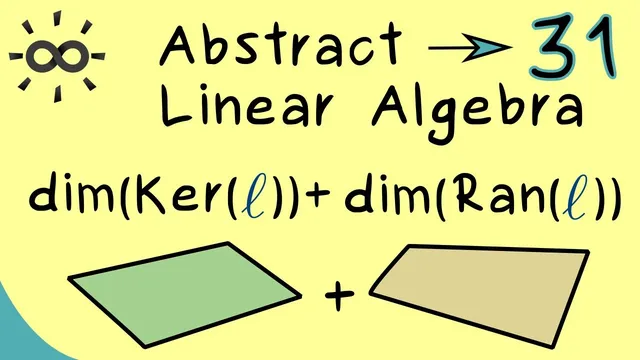
The discussion then connects these ideas to the rank–nullity theorem, a central dimension-counting result for finite-dimensional vector spaces. When V is finite-dimensional, the theorem states that dim(range(L)) + dim(ker(L)) = dim(V). Here dim(range(L)) is the rank of L, and dim(ker(L)) is the nullity. The key point is that the proof can be transferred from matrix theory: choosing bases turns L into a matrix, where the familiar rank–nullity statement holds, and the dimensions involved do not depend on which matrix representation (i.e., which bases) is chosen. That invariance is what lets the theorem hold in the abstract linear-map setting without committing to any particular coordinates.

Overall, the method replaces brute-force solving with structural criteria: check whether B lies in the range to decide existence, inspect whether the kernel is trivial to decide uniqueness, and use x0 + ker(L) to describe all solutions when they exist. The dimension relationship then quantifies how much freedom the kernel provides and how much of W the map can reach.