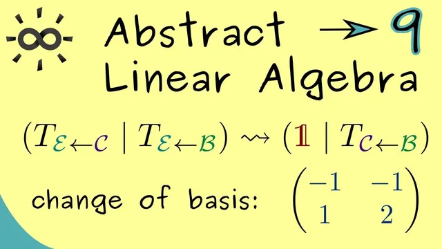
Abstract Linear Algebra 9 | Example for Change of Basis

TL;DR

A change-of-basis matrix converts coordinate representations of the same vector between two bases while the vector itself stays the same.

Briefing Cornell Notes

Briefing

Change-of-basis matrices let the same vector in an abstract vector space be represented in different bases, and the key practical takeaway is how to compute one efficiently without explicitly inverting another matrix. In

R^2, the setup starts with two bases: B = {(1,2), (3,4)} and C = {(1,0), (2,2)}. The goal is to find the change-of-basis matrix T_{C←B} that converts coordinates of a vector from basis B to coordinates in basis C. Since both bases live in R^2, the change-of-basis matrix is a 2×2 invertible matrix.

To compute T_{C←B}, the method introduces the canonical (standard) basis e = {(1,0), (0,1)} as an intermediate reference. Because the canonical basis is already expressed in standard coordinates, the transformation from B to e is straightforward: the matrix T_{e←B} is formed by placing the basis vectors of B as columns, giving T_{e←B} = [[1,3],[2,4]]. Similarly, the matrix T_{e←C} is formed from the columns of C, giving T_{e←C} = [[1,2],[0,2]]. The desired change-of-basis matrix factors through the canonical basis: T_{C←B} = (T_{e←C})^{-1} · T_{e←B}.

Rather than compute the inverse directly, the approach uses an efficient “solve one system” strategy. Let X denote the unknown matrix T_{C←B}. The factorization implies a matrix equation T_{e←C} · X = T_{e←B}. This becomes a system of linear equations with two right-hand sides (one for each column of X). Gaussian elimination can be applied to all right-hand sides simultaneously, turning the left side into the identity matrix and leaving the solution directly on the right.

Carrying out elimination on the combined system with left matrix [[1,2],[0,2]] and right matrix [[1,3],[2,4]] yields the identity on the left after scaling the second row by 1/2 and eliminating the upper-right entry by subtracting twice the second row from the first. The resulting right-hand side is the unique solution matrix X, which equals T_{C←B}. With this matrix in hand, coordinate vectors can be translated from basis B to basis C in one step.

The procedure generalizes beyond R^2: in higher dimensions like R^5, the same idea holds, though the elimination work increases. The core lesson remains: compute change-of-basis matrices by solving a single linear system via Gaussian elimination, using the canonical basis as a convenient bridge, rather than relying on explicit matrix inversion.

Cornell Notes

A change-of-basis matrix converts coordinate vectors from one basis to another while representing the same underlying vector. For R^2, the method uses the canonical basis e as an intermediate reference: build T_{e←B} and T_{e←C} by placing the basis vectors as columns. The target matrix satisfies T_{e←C} · T_{C←B} = T_{e←B}. Instead of computing (T_{e←C})^{-1} explicitly, solve this matrix equation with Gaussian elimination, treating it as a linear system with multiple right-hand sides (one per column of the unknown). The solution is the unique change-of-basis matrix T_{C←B}, and the same strategy scales to higher dimensions with more elimination steps.

Why introduce the canonical basis e when B and C are already bases of R^2?

Using e provides a fixed coordinate reference where basis vectors can be written directly as standard coordinate columns. That makes T_{e←B} and T_{e←C} easy to form: each is just the 2×2 matrix whose columns are the vectors of the corresponding basis. Then the desired transformation factors through e: T_{C←B} = (T_{e←C})^{-1} · T_{e←B}, which turns the problem into a solvable linear-algebra task.

How are T_{e←B} and T_{e←C} constructed from the given bases?

Each transformation matrix is built by placing the basis vectors as columns. For B = {(1,2),(3,4)}, T_{e←B} = [[1,3],[2,4]]. For C = {(1,0),(2,2)}, T_{e←C} = [[1,2],[0,2]]. This works because the canonical basis e is the standard coordinate system, so expressing a basis in e is equivalent to writing its vectors in standard coordinates.

What equation determines the change-of-basis matrix T_{C←B}?

Let X = T_{C←B}. The factorization through the canonical basis implies T_{e←C} · X = T_{e←B}. Concretely: [[1,2],[0,2]] · X = [[1,3],[2,4]]. Solving for X gives the matrix that maps B-coordinates to C-coordinates.

How does Gaussian elimination avoid computing an explicit inverse?

Instead of calculating (T_{e←C})^{-1}, elimination is applied directly to the matrix equation T_{e←C} · X = T_{e←B}. The left side is row-reduced to the identity matrix, and the corresponding operations are applied to the right side. When the left becomes I, the right side equals X, producing T_{C←B} in one elimination run.

Why does the method treat the problem as a system with multiple right-hand sides?

X is a 2×2 matrix, so it has two columns. Each column of X satisfies the same left-matrix equation but with a different right-hand-side column. That means there are two right-hand sides (two column vectors), and Gaussian elimination can process them simultaneously, saving work compared with solving two separate systems.

Review Questions

Given B and C in R^2, how would you form T_{e←B} and T_{e←C} from their basis vectors?
Why is solving T_{e←C} · X = T_{e←B} equivalent to computing (T_{e←C})^{-1} · T_{e←B}?
In the elimination process, what does it mean to “generate an identity matrix on the left,” and how does that make the solution readable on the right?

Key Points

1
A change-of-basis matrix converts coordinate representations of the same vector between two bases while the vector itself stays the same.
2
In R^2, the change-of-basis matrix is a 2×2 invertible matrix because both bases are linearly independent and span the space.
3
Using the canonical basis e as an intermediate reference makes T_{e←B} and T_{e←C} easy to build by placing basis vectors as columns.
4
The target matrix satisfies the matrix equation T_{e←C} · T_{C←B} = T_{e←B}.
5
Solving that matrix equation via Gaussian elimination avoids explicitly computing an inverse.
6
Gaussian elimination can handle multiple right-hand sides at once, corresponding to the columns of the unknown change-of-basis matrix.
7
The same workflow generalizes to higher dimensions (e.g., R^5), with more elimination steps but the same underlying idea.

Highlights

T_{C←B} can be found by solving T_{e←C} · X = T_{e←B}, turning the change-of-basis problem into one Gaussian-elimination run.

The canonical basis e turns “expressing in standard coordinates” into a direct column-construction rule for transformation matrices.

Multiple right-hand sides arise naturally because the unknown change-of-basis matrix has multiple columns.

Topics

Change of Basis
Canonical Basis
Gaussian Elimination
Matrix Equations