Backpropagation calculus | Deep Learning Chapter 4
Based on 3Blue1Brown's video on YouTube. If you like this content, support the original creators by watching, liking and subscribing to their content.
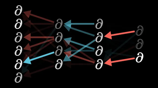
Backpropagation gradients come from applying the chain rule along the computation path from each parameter to the cost.
Briefing
Backpropagation’s calculus boils down to one practical question: how much does the cost change when a single weight or bias nudges a network’s internal numbers? The core insight is that the derivative of the cost with respect to a parameter can be written as a product of simpler derivatives using the chain rule—turning a messy network into a sequence of local sensitivities. That product tells learning algorithms exactly which parameters most strongly affect the error, enabling gradient descent to step “downhill” on the cost surface.
The walkthrough starts with an intentionally tiny network: one neuron per layer, so the last layer depends on just one weight w(L) and one bias b(L). The last neuron’s activation a(L) comes from a nonlinear function (sigmoid or ReLU) applied to a weighted sum z(L) = w(L)·a(L-1) + b(L). For a single training example with target y, the cost is C0 = (a(L) − y)^2. To find how sensitive C is to w(L), the method treats the computation as a chain: a tiny change in w(L) nudges z(L), which nudges a(L), which then changes the cost. The derivative dC/dw(L) becomes the chain rule product of three ratios: (dC/da(L))·(da(L)/dz(L))·(dz(L)/dw(L)).
Each factor has a clear meaning. The derivative dC/da(L) = 2(a(L) − y) scales with the output error: if the network output is far from the target, even small parameter tweaks can swing the cost a lot. The middle term da(L)/dz(L) is the derivative of the chosen nonlinearity, capturing how responsive the activation is to changes in its input. The last term dz(L)/dw(L) = a(L-1) shows that the weight’s influence depends on how strongly the previous neuron is “on”—a direct nod to the “neurons that fire together wire together” intuition.
The same logic applies to biases: since z(L) = w(L)·a(L-1) + b(L), the derivative dz(L)/db(L) is 1, making the bias sensitivity almost the same as the weight case. Backpropagation also reveals how error signals propagate backward: the derivative of z(L) with respect to the previous activation a(L-1) equals the weight w(L). That backward sensitivity lets the calculation iterate layer by layer, producing partial derivatives for every weight and bias.
The transcript then generalizes to multiple neurons per layer. Activations become indexed (a(L)j), and weights become edge-specific (w(L)jk) connecting neuron k in layer L−1 to neuron j in layer L. The cost sums squared output errors across neurons in the final layer. The derivative with respect to a particular weight keeps the same chain-rule structure, but the derivative with respect to an activation in layer L−1 changes because that activation affects the cost through multiple outgoing connections—so contributions from all relevant paths add together. Once those activation sensitivities are known, the same backward process yields gradients for all incoming weights and biases. The result is a systematic calculus engine for building the gradient vector that gradient descent uses to minimize cost across training data.
Cornell Notes
The key move in backpropagation calculus is rewriting dC/d(parameter) as a chain-rule product of local derivatives. In a one-neuron-per-layer network, the last layer cost is C0 = (a(L) − y)^2 with a(L) = sigmoid/ReLU(z(L)) and z(L) = w(L)a(L−1) + b(L). The derivative dC/dw(L) factors into dC/da(L) = 2(a(L)−y), da(L)/dz(L) = derivative of the nonlinearity, and dz(L)/dw(L) = a(L−1). Bias derivatives are nearly identical because dz(L)/db(L)=1. With multiple neurons, indexing expands (a(L)j, w(L)jk), and an activation’s influence on the cost sums across all paths to the output layer.
Why does the derivative of the cost with respect to a weight become a product of three terms?
What does dC/da(L) = 2(a(L) − y) tell you about learning?
How does the choice of activation function enter the gradient?
Why is dz(L)/dw(L) equal to a(L−1) in the one-neuron-per-layer example?
In a multi-neuron layer, why do derivatives with respect to earlier activations require summing multiple paths?
Review Questions
- For the one-neuron-per-layer network, write the chain-rule factorization for dC/dw(L) and identify what each factor represents.
- How does the gradient with respect to a bias b(L) differ from the gradient with respect to the weight w(L) in the simplified setup?
- In the multi-neuron case, what changes in the derivative with respect to an activation in layer L−1, and why does it require summing over multiple downstream neurons?
Key Points
- 1
Backpropagation gradients come from applying the chain rule along the computation path from each parameter to the cost.
- 2
In the last-layer one-neuron example, dC/da(L) = 2(a(L) − y), so gradient size scales with output error.
- 3
The activation function’s derivative appears as da(L)/dz(L), directly controlling how strongly errors propagate through nonlinearities.
- 4
For z(L) = w(L)a(L−1) + b(L), the weight derivative is dz(L)/dw(L) = a(L−1), linking learning to the previous layer’s activation strength.
- 5
Bias gradients are nearly the same as weight gradients because dz(L)/db(L) = 1 in the simplified model.
- 6
With multiple neurons, indexing expands (a(L)j, w(L)jk), and earlier activations affect the cost through multiple outgoing paths, so their sensitivities add up.