Backpropagation, intuitively | Deep Learning Chapter 3

TL;DR

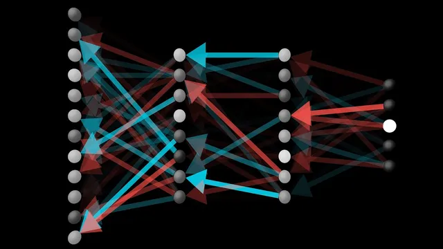
Backpropagation updates every weight and bias by following how the cost function changes with respect to each parameter.

Briefing Cornell Notes

Briefing

Backpropagation is the mechanism that turns a network’s prediction error into specific, proportionate changes to every weight and bias—so the cost function drops efficiently instead of wandering randomly. The core idea is to treat the gradient of the cost as a sensitivity map: each component of the gradient tells how strongly the cost responds if a particular weight or bias changes. In the earlier framing, that gradient lives in a huge-dimensional space, but the intuition is simple—some parameters matter far more than others, because the cost is much more sensitive to certain directions than to others.

Using a single training example (a handwritten “2”) makes the logic concrete. The network’s output activations start essentially random, so the goal isn’t to directly “fix” activations; it’s to adjust weights and biases so that the output cell for “2” rises while the other output cells fall. For the output neuron corresponding to the digit “2,” increasing its activation can happen through three cooperating levers: changing the bias, changing the weights feeding into it, or changing the activations coming from the previous layer. Weight changes are especially targeted because connections from strongly active cells in the previous layer have a larger effect—those weights multiply larger inputs, so they move the output more. This resembles a Hebbian-style intuition (“cells that fire together wire together”): stronger links tend to be those between neurons that are active together and that help produce the desired output.

The process doesn’t stop at one neuron. Every output cell has its own desired direction of change (increase for the correct digit, decrease for the others). Backpropagation aggregates these competing wishes to determine what the previous layer should do. That aggregation yields a set of desired adjustments for the activations in the layer before the output, which then translates into concrete updates for the weights and biases that produced those activations. The “back” in backpropagation comes from repeatedly running this reasoning backward through the network: each layer’s required changes are derived from how later layers’ errors depend on earlier activations.

In principle, the cost gradient for a step would be computed using every training example, then averaged. In practice, that’s too slow. The standard workaround is stochastic gradient descent: shuffle the data, split it into small mini-batches (often around 100 examples), compute gradient-based updates using one mini-batch at a time, and repeat. These updates aren’t the exact full-dataset gradient, but the repeated averaging effect across many mini-batches produces steady improvement and speeds up training dramatically.

Finally, the method’s success depends on having lots of labeled data. MNIST—handwritten digits with many pre-labeled examples—serves as a classic benchmark for demonstrating how backpropagation learns from data rather than from hand-crafted rules.

Cornell Notes

Backpropagation converts prediction mistakes into targeted updates for every weight and bias by following how the cost function changes with respect to those parameters. The gradient acts like a sensitivity vector: some parameters cause much larger cost changes than others, so updates must be scaled accordingly. For a single example (like an image of the digit “2”), the network aims to raise the “2” output activation and suppress the others; the required changes are propagated backward to determine how earlier layers’ activations and connections should shift. Because using all training examples for every update is slow, training typically uses stochastic gradient descent with mini-batches, averaging approximate gradients over many steps. Large labeled datasets like MNIST make this learning approach practical.

Why treat the gradient as a sensitivity vector rather than just a direction?

Each component of the gradient corresponds to a particular weight or bias and indicates how strongly the cost function responds to changing that parameter. If one component is much larger (e.g., 3.2 vs. 0.1 in the intuition), then the cost is far more sensitive to changes in the first parameter—about 32× more—so the update should be larger in that direction. This is why backpropagation produces not only a “which way” but also “how much” for every parameter.

For a training image of the digit “2,” what does the network try to change first?

It tries to increase the activation of the output neuron for “2” while decreasing activations for the other output neurons. Since the network can’t directly edit output activations, it adjusts weights and biases so that the forward computation yields the desired output pattern. The size of the desired change depends on how far each output is from its target (e.g., the “2” cell should move upward more than cells that are already near their target).

How do weights feeding a neuron determine the impact of changing them?

A neuron’s activation is built from a weighted sum of previous-layer activations plus a bias, then passed through an activation function (described as sigmoid or ReLU). Because weights multiply the previous activations, connections from more strongly active cells in the previous layer have greater leverage: increasing a weight tied to a bright (high-activation) input changes the neuron’s activation more than increasing a weight tied to a dim (low-activation) input.

What does “backward” mean operationally in backpropagation?

After deciding what the output layer should do (increase the correct digit, decrease the rest), the method determines what earlier layers must produce so that those output changes become possible. It aggregates the desired effects from all output neurons to compute desired changes for the previous layer’s activations. Then it repeats the same logic one layer earlier, translating those desired activation changes into weight and bias updates, moving step-by-step toward the input.

Why use mini-batches instead of computing gradients on the full dataset each step?

Computing the exact gradient using every training example at every update is computationally expensive. Mini-batch training approximates the gradient by averaging updates computed from a small subset (often around 100 examples). Although each step uses only part of the data, repeated updates across many mini-batches still drive the cost down efficiently—like a faster, noisy descent rather than a slow, exact one.

What role does MNIST play in understanding backpropagation?

MNIST provides a large supply of labeled handwritten digit images, making it feasible to train and test networks that learn via backpropagation. The transcript frames it as a common benchmark and a practical way to obtain the labeled training data required for learning at scale.

Review Questions

In what sense does the gradient provide both direction and magnitude for parameter updates?
How does the desired change in output activations for one training example translate into updates for earlier layers?
Why does stochastic gradient descent with mini-batches still converge toward a low-cost solution despite using approximate gradients each step?

Key Points

1
Backpropagation updates every weight and bias by following how the cost function changes with respect to each parameter.
2
The gradient’s components act as sensitivity scores, indicating which parameters most strongly affect the cost.
3
For a labeled example, the network targets higher activation for the correct output neuron and lower activation for the others.
4
Weight updates are more effective when they connect to strongly active neurons in the preceding layer because those weights multiply larger inputs.
5
Backpropagation works backward by aggregating desired effects from all output neurons to determine needed changes in earlier-layer activations.
6
Exact full-dataset gradient computation per step is too slow, so training uses stochastic gradient descent with mini-batches and averages approximate gradients over time.
7
Large labeled datasets such as MNIST are crucial for making backpropagation-based learning practical.

Highlights

Backpropagation turns error into proportionate parameter updates by treating the gradient as a sensitivity vector over weights and biases.

Raising the “2” output neuron isn’t done directly; weights and biases are adjusted so the forward pass produces the desired activation pattern.

Connections from more active neurons in the previous layer have larger impact because they multiply larger inputs.

Mini-batch stochastic gradient descent speeds training by using averaged approximate gradients instead of the full-dataset gradient each step.

MNIST is highlighted as a standard source of labeled digit images that makes backpropagation demonstrations possible.

Topics

Backpropagation
Gradient Sensitivity
Neural Network Training
Stochastic Gradient Descent
MNIST

Mentioned

ReLU
MNIST