Bayes theorem, the geometry of changing beliefs

Bayes’ theorem is presented as a disciplined way to update beliefs when new evidence arrives—without letting that evidence “decide” everything from scratch. The core lesson is that evidence restricts the space of possibilities, and the updated probability depends on both the starting point (prior beliefs) and how diagnostic the evidence is (likelihoods). That combination explains why people can make confident judgments that clash with probability: they often ignore the base rate, the underlying ratio of how common each hypothesis is.

The explanation begins with the classic “Steve” scenario used by Daniel Kahneman and Amos Tversky. Steve is described as shy, tidy, and detail-oriented. Asked whether Steve is more likely a librarian or a farmer, most people choose “librarian” because the description matches a stereotype. The probabilistic critique is not about stereotypes being “right” or “wrong,” but about failing to incorporate the base rate—Kahneman and Tversky cite a U.S. ratio of roughly 20 to 1 for farmers versus librarians. When that ratio is included, even a description that seems four times more likely for librarians can still yield a librarian probability under 50% because there are so many more farmers.

From there, the transcript generalizes the reasoning into Bayes’ theorem. A hypothesis H (e.g., “Steve is a librarian”) is assigned a prior probability P(H) based on base rates. New evidence E (the description) then has a likelihood P(E|H): how often that evidence appears if the hypothesis is true. The complementary likelihood P(E|¬H) captures how often the same evidence would appear if the hypothesis is false. Bayes’ theorem combines these pieces into the posterior probability P(H|E)—the belief after seeing the evidence—by weighting the hypothesis by its prior and likelihood, then normalizing by the total probability of the evidence.

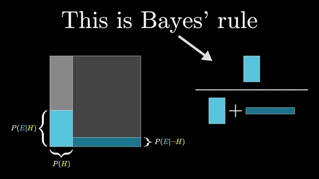
To make the computation intuitive, the transcript discourages memorizing the formula and instead encourages a geometric “area” diagram. The entire space of possibilities is treated like a 1×1 square. The hypothesis occupies a vertical slice with width P(H). Evidence restricts the square into a “wonky” subset, and the updated belief becomes the fraction of the restricted region that lies inside the hypothesis slice. When likelihoods for H and ¬H are similar, the restriction doesn’t change the proportion much; when they differ sharply, the posterior shifts substantially.

The discussion broadens beyond Bayes by revisiting another Kahneman–Tversky finding about probability judgment errors using the Linda problem. People often overestimate the likelihood of a conjunction (“bank teller and feminist movement active”) when asked in percentages, but the error disappears when the question is reframed as counts out of 100. The transcript links this to intuition: representative samples and geometric proportions help people reason about probability as proportions rather than vague uncertainty.

Finally, it returns to “Steve” and notes that debates about the experiment often hinge on context—what population the base rate should come from, and what likelihoods should be assumed. Even so, the takeaway remains consistent: evidence should update beliefs by combining prior information with how diagnostic the evidence is, rather than replacing prior beliefs with the evidence alone.