Binomial distributions | Probabilities of probabilities, part 1

TL;DR

Treat each seller’s quality as an unknown success rate S, with each review an independent positive/negative draw.

Briefing Cornell Notes

Briefing

Online ratings tempt buyers to treat “% positive” as a direct measure of quality, but the number of reviews changes what that percentage really means. A seller with 100% positives from 10 reviews can be less trustworthy than a seller with 96% from 50 reviews, because small samples make extreme outcomes far more likely. The central task is turning that intuition into a rational rule: how to trade off the confidence gained from more data against the fact that the observed percentage might be inflated or deflated by chance.

A simple rule of thumb is introduced first: pretend there were two additional reviews—one positive and one negative—so a rating of 10/10 becomes 11/12 (91.7%). For 48/50 positives, the adjusted estimate becomes 49/52 (94.2%), and for 187/200 it becomes 187+? leading to 187/202 (92.6%). Under this “rule of succession,” the second seller (96% with 50 reviews) comes out best, even though the first seller’s displayed rating is higher.

To justify such behavior quantitatively, the discussion sets up a probabilistic model. Each seller has an unknown underlying success rate S: the probability any given experience is positive. Reviews are treated as independent draws from this success rate. The observed counts—say 48 positive and 2 negative out of 50—are then modeled as outcomes of a binomial process. If S were known, the probability of seeing exactly those counts would follow the binomial distribution: “(50 choose 48) times S^48 times (1−S)^2.” This formula matters because it tells how plausible different values of S are given the data.

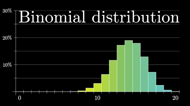
The binomial distribution is then examined from two angles. First, for a fixed S (like 0.95), simulations show that getting an extreme result such as 10 out of 10 positives is not rare—around 60% of the time in the example—so the data alone doesn’t prove the seller is truly perfect. Second, for fixed data (like 48 out of 50), the binomial probability as a function of S peaks near the observed proportion (around 0.96) but falls off quickly as S moves away. With more data, the curve becomes narrower and more concentrated, reflecting increased confidence.

A key tension is highlighted: the binomial curve’s peak corresponds to the most likely S, but that does not automatically translate into a personal probability of having a good experience. For 10/10 positives, the likelihood keeps increasing as S approaches 1, yet no buyer should conclude a 100% guarantee. The missing step is converting “probability of the data given S” into “probability of S given the data,” which requires Bayes’ rule. That transition is deferred to the next part, where Bayesian updating and continuous probability distributions are brought in.

Cornell Notes

The ratings problem is modeled by assuming each seller has an unknown success rate S: the probability a single experience is positive. Given a fixed S, the number of positive reviews out of N follows a binomial distribution, with probability proportional to (N choose k)·S^k·(1−S)^(N−k). This lets buyers quantify how likely different S values are after observing counts like 48 positives and 2 negatives. But the binomial likelihood’s peak (the most likely S) is not the same as the buyer’s probability of a good experience, especially when small samples make extreme outcomes plausible. Converting from “P(data|S)” to “P(S|data)” requires Bayes’ rule, which comes next.

Why can a 100% rating from 10 reviews be less convincing than a 96% rating from 50 reviews?

Because small samples make extreme outcomes common even when the true success rate is not 100%. Under the model, each review is an independent draw with success probability S. If S were 0.95, the chance of seeing 10 positives in 10 trials is S^10 = 0.95^10, which is substantial; simulations in the transcript show about 60% of length-10 sequences yield 10/10. So “10/10” doesn’t strongly pin down S near 1.

If the true success rate S were known, how do you compute the probability of seeing 48 positive and 2 negative reviews out of 50?

Use the binomial distribution: P(k=48 positives | S) = (50 choose 48)·S^48·(1−S)^2. The combinatorial factor (50 choose 48) counts the number of distinct sequences with 48 positives and 2 negatives, and independence allows multiplying S for each positive and (1−S) for each negative. The transcript notes that for S=0.95 this matches simulation (about 26.1% for 48/50).

What does the binomial curve look like when you fix the data and vary S?

For fixed counts (like 48 positives out of 50), the likelihood as a function of S peaks near the observed proportion (around 0.96). It drops toward 0 as S approaches 1 because then seeing any negatives becomes impossible, and it also drops quickly when S is much smaller (e.g., around S=0.8 the transcript describes the event as exceedingly rare). With more data (e.g., 480 positives and 20 negatives), the curve stays centered near the same proportion but becomes narrower and more concentrated, reflecting higher confidence.

Why doesn’t the peak of the binomial likelihood automatically give the buyer’s probability of a good experience?

The peak tells which S makes the observed data most likely, not what probability the buyer should assign to future outcomes. For 10/10 positives, the likelihood increases as S approaches 1, so the most likely S is near 1, but that doesn’t justify claiming a 100% chance of a good experience. The buyer needs a probability distribution over S that accounts for uncertainty, then uses it to predict future success.

What mathematical step is needed to turn “P(data|S)” into “P(S|data)”?

Bayes’ rule. The transcript emphasizes that the binomial formula provides P(data given S), but the decision requires P(S given the observed data). That conversion is postponed to the next part, where Bayesian updating and continuous probability distributions are introduced.

How does Laplace’s rule of succession relate to the “add two imaginary reviews” idea?

The transcript presents a rule: add one positive and one negative pseudo-count, effectively adjusting k out of N into (k+1)/(N+2). For 10/10, this becomes 11/12 (91.7%); for 48/50, it becomes 49/52 (94.2%); and for 187/200, it becomes 187/202 (92.6%). This acts like a particular Bayesian prior choice, producing a conservative estimate that avoids over-trusting extreme small-sample ratings.

Review Questions

Given observed counts k positives out of N, write the binomial likelihood in terms of S and explain what each factor represents.
Explain why increasing the number of reviews makes the binomial likelihood curve narrower even if the observed proportion stays the same.
In the 10/10 example, why is it unreasonable to treat the likelihood peak near S=1 as a literal 100% probability of future success?

Key Points

1
Treat each seller’s quality as an unknown success rate S, with each review an independent positive/negative draw.
2
Use the binomial distribution to compute P(data|S) for observed counts like 48 positives and 2 negatives out of 50.
3
Small samples make extreme outcomes plausible: even with S=0.95, 10/10 positives can occur frequently.
4
For fixed data, the binomial likelihood as a function of S peaks near the observed proportion but falls off sharply away from it.
5
More data concentrates the likelihood around the observed proportion, increasing confidence about S.
6
The decision requires converting P(data|S) into P(S|data), which is done with Bayes’ rule rather than reading off the likelihood peak.
7
Laplace’s rule of succession corresponds to adding one positive and one negative pseudo-count, yielding conservative adjusted success-rate estimates.

Highlights

A 10/10 rating doesn’t imply S=1; under S=0.95, 10/10 positives is still plausibly common.

The binomial likelihood for k positives out of N is (N choose k)·S^k·(1−S)^(N−k), combining combinatorics with independence.

With more reviews, the likelihood curve tightens around the observed proportion, reflecting reduced uncertainty.

The likelihood peak is not the same as the buyer’s probability of future success; Bayesian updating is required.

Laplace’s rule of succession turns k/N into (k+1)/(N+2), favoring sellers with enough data rather than only high displayed percentages.

Topics

Binomial Distribution
Bayesian Updating
Laplace Rule of Succession
Probability of Probabilities
Likelihood vs Prediction

Mentioned

John Cook