But how do AI images and videos actually work? | Guest video by Welch Labs
Based on 3Blue1Brown's video on YouTube. If you like this content, support the original creators by watching, liking and subscribing to their content.
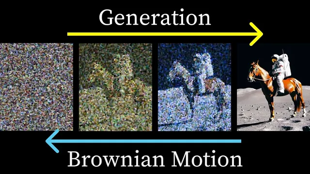
Diffusion generation starts from random noise and iteratively refines it using a learned transformer, gradually transforming structure over many steps.
Briefing
Text-to-image and text-to-video systems work because diffusion models can be understood as reversing a physics-like random process—then steering that reversal using a learned “shared space” between language and vision. The payoff is practical: the same geometric ideas that connect diffusion to Brownian motion also yield algorithms that generate sharper images faster, and they explain why prompts can reliably shape what comes out.
The walkthrough starts with a hands-on look at how a diffusion video model turns noise into structure. Generation begins by sampling a random video—pixel intensities chosen at random—then repeatedly feeds that partially structured output through a transformer. Each iteration adds a new refinement step: the result stays mostly noise early on, but gradually accumulates coherent motion and scene details. Even when the prompt is reduced to nothing, the model still produces a coherent video, showing that the core mechanism is learning a powerful prior over plausible visual worlds; prompts then act as guidance rather than full instructions.
The physics connection comes next. Diffusion models are trained by corrupting real images with increasing noise until they become nearly destroyed, then learning how to reverse that corruption. A naive “one-step denoising” intuition doesn’t match how modern systems are trained. Instead, the DDPM approach trains the network to predict the total noise added to the original image, not just the noise removed in a single step. In a simplified 2D toy setting, adding noise corresponds to a random walk; reversing it means learning a direction field that points back toward the data distribution. Crucially, the learned direction depends on the diffusion time, so conditioning on time lets the model learn coarse structure when noise is high and fine structure as noise vanishes.
Two practical surprises follow from this view. First, adding random noise during generation (as in DDPM sampling) improves sharpness. Without those stochastic steps, trajectories collapse toward an average of the training data—often producing blurry results—because the model’s learned vector field behaves like a mean-seeking estimator early in the reverse process. Second, later work shows that the same target distribution can be reached without random steps by converting the stochastic process into an equivalent deterministic one. DDIM achieves this by using differential-equation machinery (stochastic differential equations and the Fokker–Planck connection) to match the final distribution while reducing the number of steps.
Prompting enters through CLIP, which learns a shared embedding space where matching image–caption pairs align and mismatched pairs repel using a contrastive objective and cosine similarity. CLIP alone maps text and images into vectors but can’t generate. Diffusion fills that gap: the text embedding can condition the denoising process so the reverse diffusion trajectory lands on images consistent with the prompt. OpenAI’s DALL·E 2 (via unCLIP) is described as training a diffusion model to invert CLIP’s image encoder, yielding strong prompt adherence.
Conditioning alone still isn’t enough for tight control. Classifier-free guidance fixes this by combining an unconditional vector field (no text/class) with a conditioned one, then amplifying the difference. The result is that increasing the guidance scale makes details “grow” toward what the prompt specifies. For video, WAN’s approach extends the idea with negative prompts—explicitly listing unwanted features—then subtracting the negative-conditioned direction to steer away from artifacts like extra fingers or backward walking. The overall message is that diffusion’s physics-inspired geometry, combined with language-vision embeddings and guidance tricks, turns language into a controllable steering signal for a learned generative process.
Cornell Notes
Diffusion models generate images and videos by starting from random noise and iteratively reversing a noise-corruption process. The key insight is that this reversal can be interpreted as running Brownian-motion-like random walks backward in a high-dimensional space, guided by a learned time-dependent vector field (a “score function”). DDPM training predicts total noise added to the original sample, and conditioning on diffusion time lets the model learn both coarse and fine structure. During sampling, adding noise prevents collapse toward the dataset mean (which otherwise produces blur), while later methods like DDIM remove stochastic steps to reach the same final distribution more efficiently. Prompt control comes from CLIP-style embeddings plus classifier-free guidance, which amplifies the difference between unconditional and conditioned denoising directions; negative prompts further steer away from specific artifacts.
Why does diffusion generation start from pure noise, and what changes across iterations?
What does CLIP learn, and why is it useful for prompting diffusion models?
Why doesn’t the “denoise one step at a time” intuition match DDPM training?
Why does adding random noise during DDPM sampling improve sharpness?
How does DDIM generate images deterministically without changing the final distribution?
How does classifier-free guidance make prompts “stick” better than conditioning alone?
Review Questions
- In the DDPM framework, what exactly is the network trained to predict: the denoised image at each step or the total noise added to the original sample? Why does that matter?
- Explain the role of diffusion time conditioning in learning a time-varying vector field. What changes in the learned directions as time approaches 0?
- Why does removing the random noise injection during DDPM sampling tend to produce blurry outputs, and how does DDIM address efficiency without changing the final distribution?
Key Points
- 1
Diffusion generation starts from random noise and iteratively refines it using a learned transformer, gradually transforming structure over many steps.
- 2
Diffusion models can be interpreted as reversing Brownian-motion-like random walks in high-dimensional space using a time-dependent learned vector field.
- 3
DDPM training predicts total noise added to the original sample (not just one-step denoising), improving learning efficiency through reduced variance.
- 4
Adding random noise during DDPM sampling prevents collapse toward the dataset mean, which otherwise produces blur.
- 5
DDIM achieves faster, deterministic sampling by using an equivalent differential-equation formulation that preserves the final distribution.
- 6
Prompt control comes from combining CLIP-style text embeddings with diffusion conditioning, then strengthening steering via classifier-free guidance (and optionally negative prompts).