But what is a convolution?

TL;DR

Convolution of two discrete sequences produces a new sequence where each output entry is a sum of products over all index pairs that add to a fixed offset.

Briefing Cornell Notes

Briefing

Convolution is the mathematical “mixing” operation that turns two lists (or two functions) into a new list by multiplying aligned pairs and summing them—an idea that starts in probability, becomes a workhorse in image processing, and ultimately enables fast algorithms like FFT-based convolution.

The core definition is built from a simple probability picture: roll two dice and ask for the chance of each possible sum. With fair dice, counting how many outcome-pairs land on each diagonal in a grid reveals the distribution. The same question can be reframed by flipping one list of probabilities and sliding it across the other; each shift lines up pairs whose indices add to a fixed value. When the dice are not uniform, the probability of a particular sum becomes a sum of products: for each way to write the sum as i+j, multiply the probability of i on one die by the probability of j on the other, then add across all such pairs. That “sum of products across index offsets” is convolution in discrete form.

From there, convolution generalizes naturally beyond dice. In a 1D moving average, a short kernel (for example, five values each equal to 1/5) slides across a longer signal; at each position, the output is the weighted sum of the nearby inputs. The weights determine how much each neighbor contributes, so the result is a smoothed, simplified version of the original data. In two dimensions, the same mechanism blurs images: a small 3×3 or 5×5 kernel is multiplied against the pixels under it, channel by channel (RGB treated as three small vectors), producing a new pixel value. A Gaussian-shaped 5×5 kernel emphasizes the center and downweights edges, creating blur that mimics the optical effect of defocus.

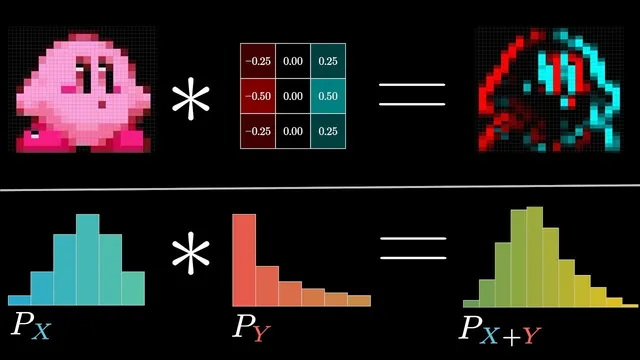
Convolution also captures structure, not just smoothing. Using kernels with positive and negative values can produce edge detection: when the kernel sums to zero, uniform regions cancel out, while changes across the image create strong positive or negative responses. Rotating the kernel changes which direction of edges are emphasized—vertical edges for one orientation, horizontal edges for another—so a carefully chosen “nucleus” (kernel) becomes a detector for specific visual features.

A practical complication is output size: mathematically, convolution often yields a longer array than the inputs, so implementations may crop or pad depending on the goal. Another subtlety is the kernel flip: the standard mathematical definition aligns with reversing the second sequence before sliding, even though many programming libraries hide this detail.

Finally, convolution’s computational cost motivates a major algorithmic leap. Naively, convolving two length-n sequences requires O(n²) pairwise products. But when the operation is reinterpreted through polynomial multiplication and evaluated at special points—specifically the roots of unity—FFT turns convolution into a sequence of faster steps: compute FFTs of both inputs, multiply pointwise, then apply the inverse FFT. This reduces runtime to O(n log n) while producing the same result, making convolution feasible at the scale used in real signal and image pipelines.

Cornell Notes

Convolution combines two sequences by sliding one against the other, multiplying aligned entries, and summing the products. In probability, it gives the distribution of sums from two independent random variables: each output value is a sum of products over all index pairs that add to the target. In image processing, convolving an image with a kernel produces effects like blurring (e.g., moving averages and Gaussian kernels) and edge detection (kernels with positive/negative weights that cancel on uniform regions). Although direct convolution is O(n²), FFT-based convolution computes the same result in O(n log n) by transforming to frequency-like coordinates using roots of unity, multiplying pointwise, and transforming back.

How does the “sum of products across index offsets” connect dice probabilities to convolution?

Represent one die’s probabilities as a list a1, a2, a3, … and the other die’s as b1, b2, b3, …. For a target sum n, consider all index pairs (i, j) such that i + j = n. The probability of sum n becomes the sum over those pairs of ai · bj. Visually, if one probability list is flipped and slid across the other, each shift aligns exactly the pairs that add to the same n, and each output entry is the total of the aligned products.

Why does a moving average blur data, and what role does the kernel’s weights play?

A moving average uses a short kernel whose entries sum to 1 (e.g., five values each equal to 1/5). At each position, the output is the weighted sum of nearby inputs under the kernel. Because the weights average neighboring values, rapid changes get damped while nearby values influence the result. If the kernel is centered (like a Gaussian), the center gets higher weight, producing blur that resembles optical defocus.

How can convolution detect edges rather than just blur?

Edge detection kernels often include both positive and negative weights and are designed so the kernel sums to zero. In a uniform region, the weighted sum cancels to near zero because positive and negative contributions offset. Where pixel values change, the cancellation breaks: one side of the kernel aligns with higher values and the other with lower values, producing a strong positive or negative response. Rotating the kernel changes which directional changes (vertical vs. horizontal) are emphasized.

What is the “kernel flip” issue, and why does it matter?

The mathematical convolution definition aligns with reversing (flipping) the second sequence before sliding it across the first. That flip can feel unnatural in programming, where many implementations effectively use cross-correlation instead. The key is consistency: if a library’s function flips internally (or not), the kernel must be interpreted accordingly to get the expected effect, especially for asymmetric kernels.

Why is naive convolution O(n²), and how does FFT reduce it to O(n log n)?

Naively, each output position requires multiplying and summing about n pairs, and there are about n output positions, leading to roughly n² operations. FFT-based convolution reinterprets the sequences as polynomial coefficients, evaluates them at roots of unity, and uses the FFT to do that evaluation efficiently. The convolution theorem then says: transform both sequences, multiply the transformed results pointwise, and apply the inverse transform—yielding the same convolution in O(n log n).

Review Questions

In the dice example, write the probability of getting sum n in terms of two probability lists a and b. What index pairs contribute?
What properties of a kernel (e.g., sum-to-zero, positive/negative weights) make it suitable for edge detection?
Why does FFT-based convolution produce the same output as direct convolution even though it avoids the explicit sliding-and-summing step?

Key Points

1
Convolution of two discrete sequences produces a new sequence where each output entry is a sum of products over all index pairs that add to a fixed offset.
2
Probability distributions of sums of independent discrete variables can be computed via convolution by summing products of aligned probabilities.
3
Moving averages and Gaussian blurs are convolution with kernels whose weights sum to 1, producing smoothing by weighted neighborhood averaging.
4
Edge detection emerges when kernels include positive and negative weights and often sum to zero, causing uniform regions to cancel while changes produce strong responses.
5
Convolution’s output length and the need for padding or cropping depend on the chosen implementation details and the mathematical definition.
6
The standard mathematical definition involves flipping the second sequence before sliding; many software functions may hide this by using cross-correlation conventions.
7
FFT-based convolution reduces runtime from O(n²) to O(n log n) by transforming inputs at roots of unity, multiplying pointwise, and transforming back.

Highlights

Convolution can be understood as “flip, slide, multiply aligned pairs, then sum,” which turns probability-of-outcomes lists into probability-of-sums.

A Gaussian-shaped kernel produces blur by weighting the center of a neighborhood more heavily than the edges.

Kernels with positive and negative values (often summing to zero) cancel uniform regions and therefore highlight edges.

FFT-based convolution computes the same result as direct convolution but replaces the O(n²) sliding work with O(n log n) transforms and pointwise multiplication.

Topics

Convolution Definition
Discrete Probability
Image Blurring
Edge Detection
FFT Acceleration

Mentioned

FFT
RGB
O(n)
O(n log n)
O(n^2)