But what is a Laplace Transform?

Q: Why can formulas like 1/s still be meaningful even where the integral diverges?

Complex analysis provides analytic continuation. Although the integral defining the transform may only converge on a half-plane, the resulting expression can extend uniquely to a larger domain if it remains analytic. That extension preserves differentiability and yields the same rational function (e.g., 1/s), even though the original integral does not converge on the left half-plane.

Q: How does linearity let cosine t reveal two poles?

Cosine t can be written as 0.5 e^(it) + 0.5 e^(-it). Linearity means the Laplace transform of the sum equals the sum of the transforms: 0.5·L{e^(it)} + 0.5·L{e^(-it)}. Using L{e^(at)} = 1/(s−a), this produces poles at s = i and s = −i, matching the two exponential components.

Q: In what way is the Laplace transform related to the Fourier transform?

When s is purely imaginary, the Laplace transform becomes nearly identical to the Fourier transform. The main differences are the lower integration bound (0 instead of −∞) and convention choices in the exponent. This is why the oscillatory behavior of e^(−st) on the imaginary axis connects directly to frequency-domain analysis.

TL;DR

Laplace transforms convert differentiation in time into multiplication by s in the transformed domain, turning differential equations into algebraic problems.

Briefing Cornell Notes

Briefing

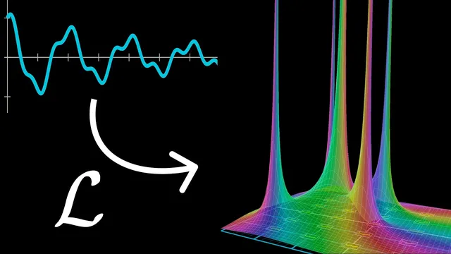
Laplace transforms turn differential-equation problems into algebra by converting derivatives into multiplication and by revealing a function’s hidden exponential components. The core insight is that when a function can be written as a sum of exponentials, the Laplace transform exposes those exponentials as “poles” in the complex s-plane—sharp spikes located at specific complex values of s. That pole structure matters because it tells you which exponential modes are present and with what weights, letting complicated time-domain behavior become simpler algebraic expressions in the s-domain.

The discussion starts by restating why exponentials are so central: differentiating an exponential e^(st) reproduces the same form, scaled by s. That property is what makes the Laplace transform powerful for differential equations—every derivative becomes multiplication by s once the transform is applied. The lesson then builds intuition for how exponentials behave when s is complex. If s has an imaginary part, e^(st) oscillates; if the real part is negative, the magnitude decays; if it’s positive, the magnitude grows. Many physics-driven functions can be decomposed into exponential pieces, such as cosine t splitting into two rotating complex exponentials e^(it) and e^(-it), and the driven harmonic oscillator ultimately involving four exponential terms.

To “see” those exponential pieces, the Laplace transform is defined as an integral: multiply f(t) by e^(-st) and integrate from t = 0 to infinity. The new variable s is complex, and the transform’s output can be viewed across the s-plane. A key preview is that if f(t) is a sum of exponentials, the transformed function develops spikes at the corresponding s-values. For example, the integral of e^(-st) alone behaves like 1/s when the integral converges (specifically, when the real part of s is positive). The integral diverges on the left half-plane because e^(-st) grows exponentially there, but the expression 1/s still provides a meaningful extension via analytic continuation.

That analytic continuation is the mathematical mechanism that reconciles “undefined” integrals with well-defined formulas elsewhere. Complex analysis is more rigid than real analysis: if a function is analytic on a region, extending it while preserving differentiability is either impossible or unique. This uniqueness lets the transform’s formula extend beyond the literal convergence region, producing a consistent pole structure.

From there, the lesson generalizes the pole idea. The Laplace transform of e^(at) becomes 1/(s − a), a simple pole at s = a. Linearity then explains how sums of exponentials map to sums of rational terms with poles at each exponential’s exponent. Applying this to cosine t, written as 0.5 e^(it) + 0.5 e^(-it), yields a transformed expression with poles at s = i and s = −i. The narrative also connects Laplace and Fourier transforms: when s is purely imaginary, the Laplace transform closely resembles the Fourier transform, differing mainly in the integration bounds and conventions.

The chapter closes by emphasizing what’s gained: poles in the s-plane reveal exponential content, and even when functions aren’t discrete sums of exponentials, Laplace transforms still express many functions as continuous superpositions of exponentials. The next step is promised as a “test drive” on an actual differential equation, after which the broader theory—reinventing the transform and relating it to Fourier inversion—will be developed.

Cornell Notes

Laplace transforms convert time-domain behavior into an s-domain function whose singularities (poles) reveal the exponential building blocks of the original signal. Exponentials matter because differentiating e^(st) reproduces the same exponential shape scaled by s, turning derivatives into multiplication in the transformed world. The transform is defined by integrating f(t)e^(-st) from 0 to infinity, which converges only when the real part of s is large enough; complex analysis then extends the result uniquely via analytic continuation. For the basic case, the transform of 1 is 1/s, and more generally the transform of e^(at) is 1/(s − a), a simple pole at s = a. Linearity lets sums like cosine t produce multiple poles, exposing its e^(it) and e^(-it) components.

Why do exponentials dominate differential-equation methods, and how does that connect to Laplace transforms?

Exponentials are special because d/dt(e^(st)) = s·e^(st). That means derivatives act like multiplication by s once the function is expressed in exponential form. Laplace transforms exploit this by converting differential operations in time into algebraic operations in the s-domain, where multiplication by s replaces differentiation.

How does the Laplace transform definition create poles in the s-plane?

The transform multiplies f(t) by e^(-st) and integrates from t = 0 to infinity. When f(t) contains an exponential piece e^(at), the integrand effectively becomes e^((a−s)t). The integral behaves like 1/(s−a) (when it converges), so the transformed function develops a simple pole at s = a. Those poles are the “spikes” that indicate which exponential rates are present.

What does convergence have to do with the left vs. right half of the s-plane?

Convergence depends on the real part of s. If Re(s) > 0, e^(-st) decays as t → infinity, so the integral can converge. If Re(s) < 0, e^(-st) grows exponentially, so the integral diverges. On the imaginary axis (Re(s)=0), the integrand oscillates without decay, so the integral does not settle to a finite value in the usual sense.

Why can formulas like 1/s still be meaningful even where the integral diverges?

Complex analysis provides analytic continuation. Although the integral defining the transform may only converge on a half-plane, the resulting expression can extend uniquely to a larger domain if it remains analytic. That extension preserves differentiability and yields the same rational function (e.g., 1/s), even though the original integral does not converge on the left half-plane.

How does linearity let cosine t reveal two poles?

Cosine t can be written as 0.5 e^(it) + 0.5 e^(-it). Linearity means the Laplace transform of the sum equals the sum of the transforms: 0.5·L{e^(it)} + 0.5·L{e^(-it)}. Using L{e^(at)} = 1/(s−a), this produces poles at s = i and s = −i, matching the two exponential components.

In what way is the Laplace transform related to the Fourier transform?