But what is the Central Limit Theorem?
Based on 3Blue1Brown's video on YouTube. If you like this content, support the original creators by watching, liking and subscribing to their content.
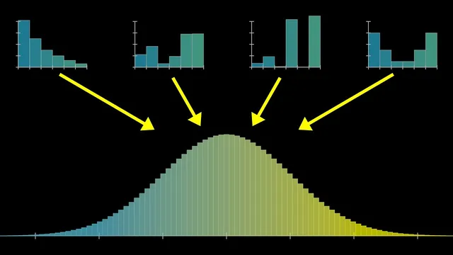
Bell-curve behavior emerges when many independent samples are added, after centering by the mean and scaling by the standard deviation.
Briefing
A single, chaotic process can be unpredictable ball-by-ball, yet the totals across many repetitions settle into a remarkably stable pattern: the bell curve. That stability is the core promise of the central limit theorem—no matter what distribution a single roll comes from (even a skewed one), the properly centered and rescaled sum of many independent samples approaches a universal normal distribution. This matters because it turns messy randomness into predictable probabilities, letting people compute ranges like “where a sum will land” with only a mean and a standard deviation.
The lesson builds the idea from a Galton board. In an idealized version, each bounce is a 50-50 choice that nudges a ball left or right by +1 or −1. After many such random choices, the final bucket corresponds to the sum of those ±1 steps. Repeating this for many balls yields a distribution of sums. With only a few steps (few rows), the shape is rough and can resemble the original asymmetries of the underlying randomness. As the number of steps grows, the distribution becomes smoother and more symmetric, converging toward a bell curve.
To generalize beyond pegs and bounces, the discussion shifts to random variables and sums. Take a random variable X (for example, the outcome of a die roll) and form a new variable by adding n independent copies of X. The central limit theorem claims that as n increases, the distribution of that sum approaches a normal distribution after centering by the mean and scaling by the standard deviation. The key quantitative ingredients are the mean and variance: the mean of a sum scales linearly with n, while the variance of a sum adds across independent variables. That means the standard deviation grows like the square root of n, so the distribution spreads out, but not as fast as the mean shifts.
The normal distribution’s exact formula is then constructed. Its shape comes from an exponential of a negative square, e^(−x^2/2), and its normalization constant is chosen so the total area under the curve equals 1. That requirement introduces the factor involving π, yielding the standard normal density: (1/√(2π))·e^(−x^2/2). From there, any normal distribution is obtained by shifting by μ (the mean) and stretching by σ (the standard deviation).
The practical payoff is illustrated with a concrete problem: rolling a fair die 100 times and finding a range that captures 95% of outcomes. The mean of one die is 3.5 and the standard deviation is about 1.71 (computed from variance 2.92). For 100 rolls, the mean becomes 350 and the standard deviation becomes 17.1. Using the common “68–95–99.7” rule, the 95% interval corresponds to roughly mean ± 2 standard deviations, giving about 316 to 384.
Finally, the theorem’s assumptions are laid out: the summed variables must be independent, identically distributed (IID), and have finite variance. Independence fails on a real Galton board because one bounce affects the next, and identical distribution can also fail because different pegs may bias outcomes. Still, broader generalizations can sometimes rescue the bell-curve behavior. The warning is that assuming normality without justification is common—and often wrong—especially when variance is infinite, where convergence to a normal distribution may fail.
Cornell Notes
The central limit theorem explains why bell curves appear so often: add up many independent samples from a single random variable, then center by the mean and scale by the standard deviation, and the resulting distribution approaches a universal normal (Gaussian) shape. The mean of the sum grows proportionally to n, while the variance adds, so the standard deviation grows like √n. The normal distribution’s density is (1/√(2π))·e^(−x^2/2), with π entering through the normalization that forces the total area under the curve to equal 1. This lets people compute probability ranges—like an approximate 95% interval using mean ± 2σ—using only the underlying mean and variance.
Why does adding many random outcomes produce a bell curve even when the original distribution is skewed?
What exactly changes when you sum n copies of a random variable—mean or spread?
How is the normal distribution formula built, and where does π come from?
How does the central limit theorem translate into a 95% range for sums like “100 die rolls”?
What do the assumptions IID and finite variance mean in this context?
Review Questions
- If X has mean μ and variance σ^2, what are the mean and variance of the sum of n independent copies of X?
- Why does the standard deviation of a sum scale like √n rather than n?
- What goes wrong with the central limit theorem if the underlying variable has infinite variance?
Key Points
- 1
Bell-curve behavior emerges when many independent samples are added, after centering by the mean and scaling by the standard deviation.
- 2
For sums of independent variables, variance adds; standard deviation grows like the square root of the number of terms.
- 3
The standard normal density is (1/√(2π))·e^(−x^2/2), with π appearing from the normalization that forces total area to equal 1.
- 4
A practical 95% interval for large sums is often approximated by mean ± 2 standard deviations using the 68–95–99.7 rule.
- 5
The central limit theorem relies on independence, identical distribution (IID), and finite variance; violating these can break normal convergence.
- 6
Real systems like a Galton board may violate IID assumptions, yet bell-curve behavior can still arise under broader generalizations—though normality should not be assumed blindly.