But what is the Fourier Transform? A visual introduction.

Fourier analysis is built around one practical question: given a signal that’s messy in time—like the air-pressure trace from a sound—how can it be broken into the pure frequencies that actually make it up? The core insight developed here is a geometric “frequency separator” that turns a time signal into a wrapped, rotating picture. When the rotation rate matches a component frequency, the wrapped shape stops canceling itself out and a clear peak appears; when it doesn’t match, the contributions average away.

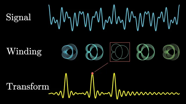
The starting example is a pure tone at 440 Hz, where air pressure oscillates smoothly up and down. Add another pure tone at a different frequency and the time trace becomes more complicated: peaks and troughs sometimes reinforce and sometimes cancel. The microphone records the combined pressure over time, but the goal is to recover the underlying frequencies. The method proposed is to treat the signal as a curve and “wrap” it around a circle. At each moment, the height of the curve becomes the radial distance from the center, producing a rotating vector-like shape in a 2D plane. A second frequency—called the “wrapping frequency”—controls how fast the curve is wound around the circle.

As the wrapping frequency changes, the wrapped curve’s center of mass shifts. For most wrapping rates, positive and negative contributions around the circle balance out, keeping the center near the origin. But when the wrapping frequency aligns with a signal component, the wrapped curve’s peaks line up on one side of the circle and troughs on the other, pushing the center of mass away from the origin. That alignment produces a sharp rise in the measured quantity (initially tracked via the sine-coordinate of the center of mass). In the simplified “Fourier approximation” picture, the most important feature is the peak at the true component frequency.

The same mechanism works when the signal contains multiple frequencies. Combining two tones—say 3 Hz and 2 Hz—creates a time-domain waveform that looks like interference. Feeding that combined signal into the wrapping-and-centering process yields a wrapped representation that looks chaotic at first, yet the center-of-mass peaks reappear precisely at the component frequencies. The crucial property is linearity in practice: applying the Fourier-like operation to each pure tone and then combining results matches what happens when the combined signal is processed directly. That’s what makes filtering possible: a high-frequency nuisance tone shows up as a peak at high frequency, and suppressing that peak removes the unwanted component.

To move from the geometric sketch to the actual Fourier transform, the explanation upgrades the 2D center-of-mass idea into complex numbers. The wrapping rotation is encoded using Euler’s formula, where exponentials of imaginary numbers represent rotation on the unit circle. The final expression becomes an integral (or, in real applications, a finite-time integral) of the signal multiplied by a complex rotating factor. The real part corresponds to the sine-coordinate-style measurement used earlier, while the imaginary part captures the complementary coordinate.

A key practical nuance is that the true Fourier transform uses only part of the integral—effectively normalizing by time length rather than scaling by it indefinitely—so the magnitude at a frequency grows when that frequency persists. The discussion ends by promising that the full transform’s deeper structure extends beyond frequency extraction, with more mathematical reach in a follow-up. A brief sponsor segment closes with a Jane Street puzzle about vector sums on a 3D surface.