Convolutional Neural Networks - Deep Learning basics with Python, TensorFlow and Keras p.3

TL;DR

CNNs classify images by extracting hierarchical features through repeated Conv2D and pooling operations.

Briefing Cornell Notes

Briefing

Convolutional neural networks (CNNs) are built to extract visual features from images by repeatedly applying convolution and pooling, then using those learned features to classify inputs like cats versus dogs. The core mechanism is straightforward: a small sliding window (commonly 3×3) moves across pixel grids, producing feature values from local regions, while max pooling downsamples by keeping only the strongest activation in each window (often 2×2). Stacking these operations gradually shifts the model from low-level patterns—edges and lines—to more complex shapes like curves and circles, and eventually to higher-level concepts that can resemble parts of animals (eyes, faces) as depth increases.

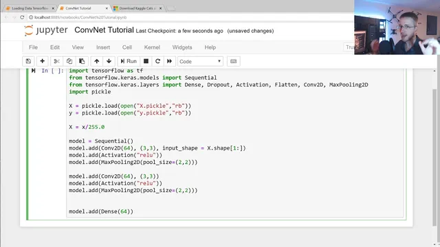
After establishing the intuition, the workflow turns into a practical TensorFlow/Keras implementation. Image data is loaded from pickled files (X and y), then normalized by dividing pixel values by 255 so inputs fall into a 0–1 range. A Keras Sequential model is assembled with a convolutional layer (Conv2D) using 64 filters and a 3×3 kernel, paired with a max pooling layer (MaxPooling2D) using a 2×2 pool size. Because convolutional layers output multi-dimensional feature maps, the model flattens those maps into a 1D vector before feeding them into a dense layer.

The architecture then adds a dense layer with 64 units and an output dense layer with 1 unit, followed by an activation step using the rectified linear family for intermediate processing (ReLU is referenced as the activation used earlier). Training is configured with model.compile using Adam as the optimizer and accuracy as the metric. The loss function is set for binary classification (the transcript mentions binary cross-entropy, with a brief confusion between “categorical” and “binary” naming), aligning with the cats-vs-dogs target.

Training uses model.fit on the normalized X and labels y, with a batch size chosen from a typical range (the transcript notes that very large batch sizes can hurt and that practical values often fall roughly between tens and a couple hundred, depending on dataset size). A validation split reserves a portion of the training data for out-of-sample monitoring—set to 10% in the run described. After training for a small number of epochs (the transcript runs 1 epoch first, then increases to 3), validation accuracy lands in the mid-to-high 70% range, with the expectation that additional epochs could push performance beyond 80% if the model keeps generalizing.

A key takeaway is how to interpret training signals: the transcript flags a “wonky” pattern where validation accuracy can temporarily exceed training accuracy, noting that this isn’t automatically fatal but should become a red flag if it persists consistently. The next step promised is TensorBoard—used to visualize training curves and diagnose issues like overfitting, instability, and misleading metrics.

Cornell Notes

CNNs classify images by learning features through repeated convolution and pooling. Convolution slides a small window (e.g., 3×3) across pixel grids to produce feature activations, while max pooling (e.g., 2×2) keeps the strongest activation in each region to downsample. In the implementation, images are loaded from pickled arrays, normalized by dividing by 255, then fed into a Keras Sequential model: Conv2D → MaxPooling2D → Flatten → Dense layers → output. The model trains with Adam and tracks accuracy using a validation split (10%). Early results reach roughly the high-70% validation accuracy after a few epochs, with guidance to watch for suspicious training/validation patterns.

How does convolution turn an image into useful features?

A convolutional layer applies a small window (commonly 3×3) across the image’s pixel grid. At each position, the window computes a value that summarizes local patterns, then the window shifts by a stride and repeats. Doing this many times produces a feature map—an organized set of activations that represent where certain visual cues appear. Early layers tend to capture simple structures like edges and lines; deeper layers combine those into more complex shapes.

What does max pooling do, and why is it paired with convolution?

Max pooling downsamples feature maps by taking the maximum value within a pooling window (often 2×2). As the window slides across the feature map, it keeps only the strongest activation in each region. This reduces spatial size, helps make the representation more robust to small shifts, and reduces computation while preserving the most salient features.

Why normalize image data by dividing by 255?

Pixel values typically range from 0 to 255. Dividing by 255 scales inputs into the 0–1 range, which stabilizes training and makes gradient-based optimization easier. The transcript performs this directly as x = x / 255 before model training.

Why does the model use Flatten before a dense layer?

Convolution and pooling output multi-dimensional tensors (height × width × channels). Dense layers expect 1D feature vectors. Flatten converts the feature maps into a single vector so the dense layers can learn from the extracted features.

What training setup choices affect performance and generalization?

The transcript uses model.compile with Adam and accuracy, and trains with model.fit using a batch size and a validation split. Batch size is discussed as a practical tradeoff: very large batches can lead to worse results, while typical values often fall in the tens to a couple hundred range depending on dataset size. Validation split (10% here) provides an out-of-sample check during training.

How should accuracy vs. validation accuracy be interpreted?

The run reports validation accuracy around the high-70% after a few epochs and notes a “wonky” situation where validation accuracy can be higher than training accuracy. That can happen early or due to sampling noise, but persistent mismatches can signal issues like data leakage, evaluation quirks, or unstable training. The transcript flags this as something to watch over multiple epochs.

Review Questions

If a CNN’s early layers learn edges and lines, what kinds of patterns are expected in later layers, and why?
What is the functional difference between convolution and max pooling, and how does each change the tensor shape?
Why might validation accuracy sometimes exceed training accuracy, and what would make that pattern concerning?

Key Points

1
CNNs classify images by extracting hierarchical features through repeated Conv2D and pooling operations.
2
Convolution uses a sliding window (e.g., 3×3) to compute local feature activations across the image.
3
Max pooling (e.g., 2×2) reduces spatial dimensions by keeping the maximum activation in each window.
4
Image inputs are normalized by dividing pixel values by 255 to stabilize training.
5
A Keras Sequential CNN typically follows Conv2D → MaxPooling2D → Flatten → Dense layers before the output.
6
Training uses Adam optimization and tracks accuracy, with a validation split (10% here) to monitor generalization.
7
Accuracy vs. validation accuracy should be monitored for suspicious patterns, especially if the gap persists across epochs.

Highlights

A 3×3 convolution window slides across pixel grids to build feature maps, while 2×2 max pooling keeps only the strongest activations.

Normalization by x/255 scales pixel inputs from 0–255 into 0–1, improving training stability.

Because convolution outputs multi-dimensional feature maps, Flatten is required before dense layers can operate.

With a simple cats-vs-dogs CNN (Conv2D + MaxPooling + Dense), validation accuracy reaches the high-70% range after a few epochs.

Validation accuracy can temporarily outperform training accuracy, but persistent “wonky” patterns are a warning sign.

Topics

Convolutional Neural Networks
Cats vs Dogs Classification
TensorFlow Keras Model
Image Normalization
Training Metrics

Mentioned

CNN
TF
Keras
Adam