Cramer's rule, explained geometrically | Chapter 12, Essence of linear algebra

Cramer’s rule gets its power from a geometric fact about determinants: when a linear transformation acts on space, every “coordinate-carrying” area (in 2D) or volume (in 3D and higher) gets scaled by the same factor—the determinant of the transformation matrix. That shared scaling lets the coordinates of the unknown input vector be recovered from the known output, without relying on dot products or orthonormal structure.

The setup starts with a linear system with two unknowns, written as a matrix transformation sending an unknown vector (x, y) to a known output (for example, −4, −2). The columns of the matrix describe where the basis directions land, so the puzzle becomes: which input vector produces the given output? When the determinant is nonzero, the transformation is invertible—each output corresponds to exactly one input.

A tempting but generally wrong idea is to recover x and y using dot products, hoping that dot products with transformed basis vectors would still equal the original coordinates. That fails because most linear transformations do not preserve angles or perpendicularity: vectors that were perpendicular can become non-perpendicular, and vectors that had positive dot products can end up with negative ones. Only special transformations—orthonormal ones—preserve dot products, making coordinate recovery via dot products work cleanly. Since typical systems aren’t orthonormal, a different invariant is needed.

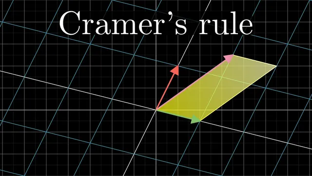
Determinants supply that invariant. In 2D, the y-coordinate can be reinterpreted as the signed area of a parallelogram spanned by the first standard basis vector (i-hat) and the unknown vector (x, y). Similarly, the x-coordinate corresponds to the signed area of the parallelogram spanned by the unknown vector and the second basis vector (j-hat). Under a linear transformation, these signed areas don’t stay fixed; they all scale by the determinant of the transformation matrix.

This scaling is the engine behind Cramer’s rule. To solve for y, one forms a new matrix by replacing the second column of the original matrix with the known output vector, then takes its determinant. Dividing that determinant by the determinant of the original matrix yields y. The same logic solves for x: replace the first column with the output vector, take the determinant, and divide by the original determinant. The determinants act like “area measurements” in the transformed space, and the determinant of the full matrix serves as the universal conversion factor back to the original coordinates.

A quick numerical check confirms the method: with a system whose relevant determinants are 6 (for the modified matrix) and 2 (for the original), the rule gives x = 3; for y, the corresponding determinant ratio gives y = 2. The argument generalizes beyond 2D by swapping parallelogram areas for signed parallelepiped volumes in higher dimensions, again relying on the determinant’s role as the common scaling factor for all those oriented volumes. The payoff is both computational and conceptual: Cramer’s rule is not the fastest method in practice, but it reveals how determinants encode the geometry of linear systems in a remarkably direct way.