DBSCAN Clustering Algorithms | Density Based Clustering | How DBSCAN Works | CampusX

DBSCAN’s core strength is that it clusters data by density—grouping together regions where points are packed closely—while automatically flagging sparse points as noise. That density-first approach matters because many real datasets don’t form neat, spherical clusters, and algorithms like k-means can break down when cluster shapes are irregular or when outliers distort centroids.

The discussion starts with why k-means often fails in practice. k-means requires the number of clusters up front, which becomes especially awkward in high-dimensional data where visual intuition is missing. Even when the “right” cluster count is guessed (for example via elbow plots), the result can be ambiguous. k-means is also sensitive to outliers: a single distant point can pull centroids away from where they should be. Finally, k-means assumes centroid-based, roughly spherical structure; when data forms non-spherical shapes, it can produce incorrect groupings.

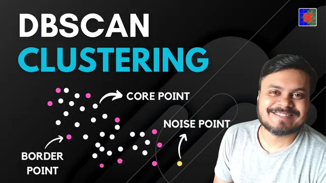
DBSCAN avoids those pitfalls by using two hyperparameters: ε (epsilon), the neighborhood radius, and MinPts, the minimum number of points required to consider a region dense. For any point, DBSCAN counts how many points fall within its ε-neighborhood. If that count is at least MinPts, the point is a core point. If the count is below MinPts but the point lies within ε of a core point, it becomes a border point. Points that are neither core nor border are labeled as noise.

The algorithm then builds clusters through the idea of density connectivity. Two points are density-connected if there exists a chain of core points linking them such that each adjacent step stays within ε. If the chain breaks—because a link passes through a non-core region or because the distance between core points exceeds ε—then the points belong to different clusters.

Operationally, DBSCAN runs in four steps. First, it sets ε and MinPts, then labels every point as core, border, or noise based on neighborhood counts. Second, it iterates over unassigned core points: each time it finds a new core point, it starts a new cluster and expands it by repeatedly adding all core points density-connected to the current cluster. Third, it assigns each border point to the cluster of its nearest core point within ε. Fourth, it leaves noise points unassigned.

A practical implementation example uses scikit-learn’s DBSCAN, fitting the model with ε and MinPts (min_samples) and reading cluster labels from the output; noise points receive a label of −1. The walkthrough also highlights how changing hyperparameters can dramatically alter results: increasing MinPts can turn previously clusterable points into noise, while increasing ε can merge clusters by expanding neighborhoods.

Finally, the advantages and limitations are laid out. DBSCAN is robust to outliers, doesn’t require specifying the number of clusters, and can find arbitrarily shaped clusters. But it is sensitive to ε and MinPts, struggles when clusters have very different densities, and doesn’t provide a direct prediction function for new points without re-running clustering. The takeaway is clear: DBSCAN is powerful for density-shaped structure, but it demands careful tuning of its two neighborhood parameters.