Deep Learning with Python, TensorFlow, and Keras tutorial
Based on sentdex's video on YouTube. If you like this content, support the original creators by watching, liking and subscribing to their content.
Keras provides high-level APIs on top of TensorFlow, making it faster to build and train neural networks without manually writing low-level TensorFlow code.
Briefing
Deep learning with Python is now far easier to start than it was a couple of years ago, thanks to high-level Keras APIs that sit on top of TensorFlow. The core takeaway is that a practical neural network workflow can be built quickly: define an architecture, normalize inputs, train with a suitable optimizer and loss function, then check whether performance holds up on unseen data.
The tutorial begins with a compact mental model of how neural networks map inputs to outputs. Inputs (for example, pixel values) connect to a hidden layer through weighted connections. Those weighted sums pass through an activation function that determines whether a neuron “fires” in a nonlinear way—moving beyond purely linear relationships. With multiple hidden layers, the model becomes a “deep” neural network capable of learning complex patterns. For classification, the output layer typically uses sigmoid or, more commonly for multi-class problems, softmax to produce a probability distribution across classes. Predictions then come from choosing the class with the highest probability (argmax).
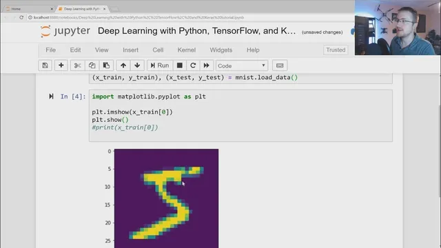
From there, the walkthrough shifts into a concrete build using TensorFlow/Keras and the MNIST dataset of 28×28 handwritten digits (0–9). The data is split into training and testing sets (X_train, Y_train, X_test, Y_test). Before training, pixel values are normalized from their original 0–255 range into 0–1 using tf.keras.utils.normalize, which makes learning easier and improves results. The model is defined as a Keras Sequential network: a Flatten layer converts the 2D image into a 1D vector, followed by two Dense hidden layers with 128 units each using ReLU (tf.nn.relu). The final Dense output layer has 10 units (one per digit) and uses softmax to output class probabilities.
Training is configured via model.compile with the Adam optimizer, a cross-entropy loss suited to sparse integer labels (sparse categorical cross entropy), and accuracy as the metric. The model is trained for a small number of epochs (three) using model.fit. Training performance is strong—around 97% accuracy after three epochs—yet the tutorial stresses that high training accuracy can hide memorization. The next step is validation/testing using model.evaluate on the test set. The results land lower than training (about 96.5% accuracy with higher loss), which is expected; the key warning is to watch for a large gap between training and validation metrics, a common sign of overfitting.
Finally, the tutorial shows how to save and reload a trained model (model.save and tf.keras.models.load_model) and how to interpret predictions. model.predict returns probability vectors (one-hot-like distributions), so argmax is used to convert them into a single predicted digit. A quick plot of a test image confirms the predicted label. The closing message points toward follow-up topics such as loading external datasets, using TensorBoard, and deeper model debugging—because real-world performance often depends on diagnosing what the model is learning and why it fails on new data.
Cornell Notes
The tutorial lays out a practical end-to-end recipe for building a Keras neural network on MNIST: define a Sequential model, normalize inputs, train with Adam and cross-entropy, and then verify generalization on a held-out test set. It starts with the core mechanics of neurons—weighted sums plus nonlinear activation—and explains why softmax outputs probabilities for multi-class classification. The MNIST model uses Flatten plus two Dense ReLU layers and a 10-unit softmax output. Training reaches about 97% accuracy in three epochs, but evaluation on test data drops to roughly 96.5%, illustrating the need to check overfitting. Predictions are probability vectors, so argmax converts them into the final digit label.
How does a neural network turn inputs into a class prediction?
Why does the tutorial normalize MNIST pixel values before training?
What architecture is used for the MNIST classifier in Keras?
What loss, optimizer, and metric are selected, and why do they matter?
How does the tutorial detect overfitting?
Why do predictions look “messy,” and how are they converted into a digit label?
Review Questions
- What role does the activation function play in enabling nonlinear relationships in a neural network?
- Why is argmax the right step after softmax outputs class probabilities?
- What training-vs-test metric pattern would most strongly indicate overfitting?
Key Points
- 1
Keras provides high-level APIs on top of TensorFlow, making it faster to build and train neural networks without manually writing low-level TensorFlow code.
- 2
Neural networks compute weighted sums of inputs and apply nonlinear activation functions; classification typically uses softmax to produce class probabilities.
- 3
For MNIST, Flatten + Dense(ReLU) layers plus a softmax output layer forms a straightforward baseline classifier.
- 4
Normalizing pixel values from 0–255 to 0–1 using tf.keras.utils.normalize improves learning and typically boosts performance.
- 5
Training optimizes loss (not accuracy), so selecting an appropriate loss function (sparse categorical cross entropy for integer labels) is crucial.
- 6
High training accuracy is not enough; evaluating on X_test with model.evaluate helps detect overfitting by comparing train and test metrics.
- 7
Predictions are probability distributions, so argmax converts them into a single predicted class label.