Differential equations, a tourist's guide | DE1

Differential equations are the language for describing change—when it’s easier to model how a system evolves than to pin down its exact state at every moment. From Newtonian mechanics to population growth and even the dynamics of affection, they formalize relationships where rates of change depend on the current values themselves. The core takeaway is that many real-world systems can be expressed as equations linking a function to its derivatives, and that this structure unlocks both qualitative insight and practical computation, even when exact formulas are out of reach.

The tour begins by distinguishing two main types: ordinary differential equations (ODEs), where the unknown depends on a single input such as time, and partial differential equations (PDEs), where the unknown depends on multiple inputs like space and time. A thrown object under gravity provides a first ODE: if y(t) is vertical position, then ÿ = −g. Solving it means “working backwards” from derivatives—integrating to recover velocity and position while using initial conditions to fix the constants. That simple example already hints at a recurring theme: differential equations often contain feedback loops where acceleration depends on position (or other state variables), not just on time.

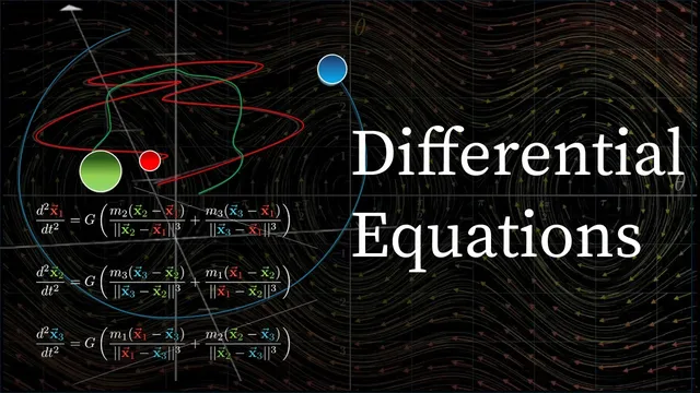
Gravity between bodies makes that feedback explicit. In the two-body gravitational setting, acceleration depends on distance, so the system becomes a coupled dance between position and velocity. More generally, physics often uses second-order differential equations, where the highest derivative appearing is the second derivative; higher-order equations involve third, fourth, or even higher derivatives. Conceptually, solving such equations is like assembling an “infinite jigsaw puzzle”: the values of the unknown at every time must fit together with their own rate-of-change constraints.

The pendulum example turns that abstraction into something concrete—and more realistic than the standard small-angle sine-wave story. The true restoring acceleration involves sin(θ), not θ, so the pendulum’s period lengthens for larger swings and the motion stops resembling a pure sine wave. With damping included (modeled as a term proportional to angular velocity), the resulting nonlinear differential equation becomes “juicy”: analytic solutions are either extremely complicated or unavailable in closed form. That limitation pushes the focus from exact solving to understanding the dynamics directly from the equations.

To build that understanding, the discussion shifts from plotting θ versus time to using phase space: a two-dimensional state space with axes (θ, θ̇). Each point represents a complete snapshot of the system, and the differential equation induces a vector field that shows how the state moves. Trajectories spiral toward stable fixed points when damping is present, and changing parameters like the air-resistance coefficient μ changes how quickly the spiral tightens. This same phase-space approach generalizes beyond pendulums: the three-body problem expands the state space dramatically (18 dimensions for positions and momenta), and the stability question becomes a matter of whether nearby trajectories contract or expand.

Finally, when exact solutions are unavailable, numerical simulation offers a practical path: step forward in time using small increments Δt, repeatedly updating θ and θ̇ based on the differential equation. The tour closes by connecting these modeling limits to chaos theory—small measurement errors can cause trajectories to diverge rapidly, making long-term prediction unreliable even when the equations are known. The result is a sobering but motivating message: the complexity of nature isn’t hidden; it lives inside the math itself.