Diffusion Policy Controlling Robots - Part 2

Diffusion policy for robot control turns a noisy guess of future actions into a smooth, goal-reaching trajectory by repeatedly denoising an action sequence—using robot observations as conditioning. Instead of producing a single next move, the model predicts an entire horizon of actions (e.g., 16 steps of a 2D end-effector position), then the robot executes only part of that sequence in a receding-horizon loop: take new observations, re-run the diffusion denoising process, and continue until the task goal is met. This matters because it reframes robot control as conditional generative modeling over action trajectories, giving a mechanism to enforce temporal consistency and reduce “jitter” that can happen when predicting one action at a time.

The core setup uses a conditioned diffusion process that ingests observations—typically two recent state vectors in the push-T example—and refines a sequence of future actions over K diffusion iterations. The action space is position control: where the end-effector should be to move the block (the “T”) toward a target location. Visualizations in the discussion describe how early diffusion steps correspond to far-future, high-uncertainty action distributions (shown in warmer colors), while later steps concentrate into a coherent trajectory that achieves the goal.

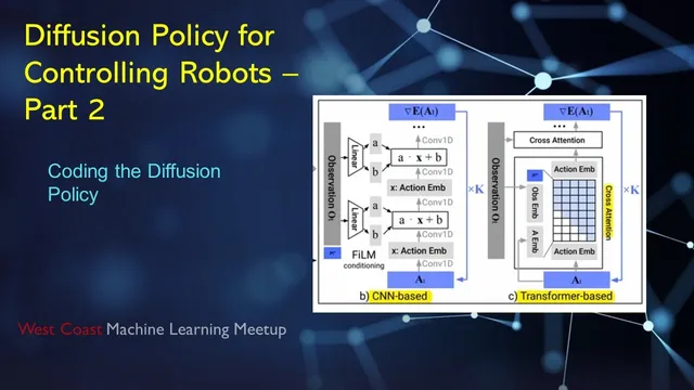
Conditioning is implemented in two architectural styles. In the CNN-based variant, observations are encoded with a U-Net backbone and injected via FiLM (feature-wise linear modulation): intermediate feature maps are scaled and shifted using learned functions of the observation embedding. In the Transformer-based variant, observations and actions are embedded and combined through masked attention, again iterating through diffusion steps to denoise the action sequence.

A major conceptual thread during the session is what diffusion models are actually learning. Rather than directly outputting probabilities over actions, diffusion policy trains a network to predict the noise (equivalently tied to the score function, i.e., the gradient of the log probability of the action distribution). That distinction is tied to training stability: compared with an implicit energy-based policy (energy/unnormalized probability estimation), the score-based formulation avoids estimating the normalizing denominator, which can make optimization more stable. The tradeoff is inference cost: generating actions requires iterative denoising, though faster samplers and differential-equation solvers can reduce the number of steps.

The practical walkthrough then shifts to data and code. Training relies on a limited set of human demonstrations—about 200 manual episodes in the push-T setup—split into many training fragments. Each fragment uses two observations and asks the model to predict the next 16 actions. For real-world data, demonstrations are collected with a space mouse and recorded with cameras including an overview camera and a wrist camera for fine positioning. The discussion also clarifies how the simulation environment works (a 2D physics model with collision/overlap-based rewards) and how the training loop normalizes observations and actions to a -1 to +1 range, samples diffusion time steps and noise, and trains a conditional 1D U-Net with an MSE loss between predicted and true noise.

Finally, the session highlights how diffusion’s “mode decisions” appear to happen early when noise is high: exploratory, multi-modal behavior can emerge at early diffusion steps, but later steps collapse into a committed trajectory, enabling smooth, goal-directed motion rather than oscillation between alternatives.