Dot products and duality | Chapter 9, Essence of linear algebra

Dot products don’t just measure “how much two vectors point together”—they secretly encode a linear transformation. That deeper link, revealed through duality, explains why the coordinate formula matches projection geometry and why dot products naturally appear when linear maps collapse higher-dimensional space down to a number.

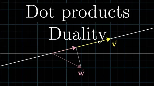
The usual entry point into dot products is numerical: for vectors of the same dimension, multiply corresponding coordinates and add the results. For example, (1,2)·(3,4)=1·3+2·4, and (6,2,8,3)·(1,8,5,3)=6·1+2·8+8·5+3·3. Geometrically, the same quantity can be read as follows: project one vector onto the line through the origin in the direction of the other, take the length of that projection, and multiply by the length of the original vector. The sign tracks whether the projection points along the same direction (positive), is perpendicular (zero), or points opposite (negative).

That geometric picture can feel asymmetric—projecting w onto v looks different from projecting v onto w—yet the dot product is symmetric. The symmetry becomes intuitive once scaling is considered. If v is scaled by a constant (say 2v), then under the “project w onto v” viewpoint the projection length stays the same while the vector being projected onto doubles; under the “project v onto w” viewpoint the projection length doubles while the target vector’s length stays fixed. Either way, the dot product doubles, so the order doesn’t change the outcome.

The real puzzle is why the coordinate recipe has anything to do with projection at all. The answer comes by stepping into linear transformations from 2D to 1D (the number line). A linear map that takes a 2D vector to a single number is fully determined by where it sends the basis vectors i-hat and j-hat; those images become the columns of a 1×2 matrix. Matrix multiplication in this setting looks strikingly like a dot product: multiplying a 1×2 matrix by a 2D vector is equivalent to dotting the vector with the “tilted” version of that matrix.

To make the connection concrete, the number line is embedded diagonally in the plane. Projecting a 2D vector onto this diagonal line defines a linear function that outputs a number. The key geometric object is the unit vector u-hat pointing toward the embedded point labeled 1. When i-hat and j-hat are projected onto the diagonal number line, the resulting numbers are exactly the x- and y-coordinates of u-hat. Those coordinates form the 1×2 matrix for the transformation, so applying the transformation to any vector becomes identical to taking the dot product with u-hat. Scaling u-hat by 3 scales the transformation by 3 as well, yielding the general rule: dotting with a non-unit vector corresponds to projecting onto its direction and then scaling by the vector’s length.

This is the essence of duality in linear algebra: a vector can be viewed as encoding a linear transformation to the number line, and a linear transformation to the number line corresponds back to a specific vector. In that light, the dot product is more than a geometric test for direction—it’s a translation mechanism between vectors and transformations, letting arrows in space stand in for linear maps.