Evaluate (4) - Troubleshooting - Full Stack Deep Learning

TL;DR

Use evaluation results to prioritize model improvements; interpret performance through bias–variance decomposition rather than relying on a single metric.

Briefing Cornell Notes

Briefing

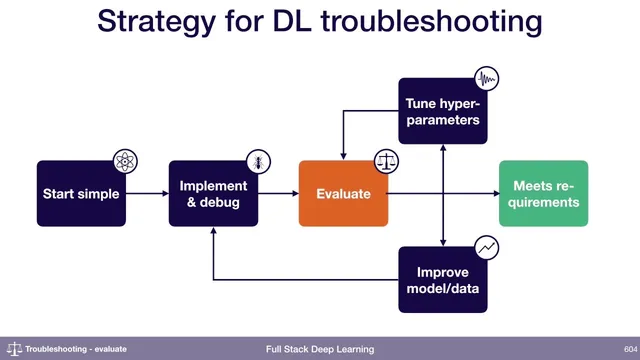
Model improvement starts with evaluation, not guesswork: once a team is reasonably confident the model is bug-free, the next move is to measure performance and use those measurements to decide what to fix. A practical framework comes from bias–variance decomposition, which breaks final test error into components that point to different failure modes. In a typical learning-curve pattern, training error decreases toward a target (often near “human level” performance), validation error sits higher than training error, and test error sits higher than validation error. Bias–variance decomposition interprets the gap structure: irreducible error reflects the best achievable baseline (e.g., human-level or target performance), avoidable bias corresponds to underfitting and is measured by how much worse training error is than expected, and variance corresponds to overfitting and is measured by how much worse validation error is than training error. A further gap between validation and test error can indicate overfitting to the validation set itself.

A key assumption underlies this decomposition: training, validation, and test sets must come from the same data distribution. When that assumption breaks—such as pedestrian detection performed in daytime for training but evaluated mostly at night—the error decomposition needs an extra term. The recommended fix is to use two validation sets: one sampled from the training distribution and another sampled from the test distribution. This adds a measurable “distribution shift” component: if test-distribution validation error is significantly worse than training-distribution validation error, the model is losing performance because the deployment environment differs from what it saw during training.

The transcript illustrates how these signals guide diagnosis using a pedestrian detection example with a goal performance of 1%. If training error is 20%, the model is far from the target, implying massive underfitting (training error minus goal). If validation error is 27%, the model is also overfitting (validation error minus training error). If test error then matches validation error, the situation looks relatively consistent—suggesting the main issues are bias and variance rather than heavy overfitting to the validation set.

After laying out the evaluation logic, the discussion turns to implementation and data strategy. For numerical or shape-related bugs, the advice is a hybrid approach: be careful during implementation (for example, scrutinize operations that can cause numerical instability), but also aim to overfit a single batch quickly. That fast check often catches issues sooner than line-by-line code review. For distribution shift when test-distribution data is scarce, the guidance is to still create a test-distribution validation set—splitting the limited samples (e.g., 100 points total into 50 for validation and 50 for the final test set, or similar ratios). Finally, when choosing between hyperparameter settings, the preference depends on whether the validation set truly matches the deployment distribution; if it does, the lowest validation error is the best automated choice, but if validation is biased toward the training distribution, that choice can mislead and lead to worse real-world performance.

Overall, the core takeaway is that evaluation should produce actionable error components—bias, variance, irreducible error, and distribution shift—so improvement work can be prioritized instead of randomized.

Cornell Notes

Bias–variance decomposition turns test error into interpretable parts: irreducible error (baseline limit), bias/underfitting (training error worse than expected), variance/overfitting (validation error worse than training error), and potentially extra overfitting to the validation set (test error worse than validation error). This framework assumes train/validation/test come from the same distribution. When deployment differs (e.g., day-trained pedestrian detection evaluated at night), using two validation sets—one from the training distribution and one from the test distribution—adds a distribution-shift term that quantifies the gap. Even with limited test-distribution data, creating a small validation set from that distribution is still emphasized to measure overfitting and shift. Fast debugging also matters: overfitting a single batch quickly can reveal numerical or shape bugs sooner than careful code reading alone.

How does bias–variance decomposition translate learning-curve gaps into specific problems to fix?

It decomposes final test error into irreducible error plus avoidable bias and variance (and sometimes a validation-to-test overfitting term). Irreducible error is the baseline limit (e.g., human-level/target performance). Bias/underfitting shows up when training error is much worse than what the baseline suggests. Variance/overfitting shows up when validation error is worse than training error by a noticeable margin. If test error is worse than validation error, that can indicate overfitting to the validation set itself.

What breaks the standard bias–variance decomposition, and how is it handled?

The decomposition assumes training, validation, and test sets come from the same data distribution. When they don’t—like pedestrian detection trained on daytime images but tested mostly at night—the validation/test gap can reflect distribution shift rather than model capacity issues. The fix is to use two validation sets: one sampled from the training distribution and one sampled from the test distribution. The difference between these validation errors becomes a measurable distribution-shift term.

In the pedestrian detection example, what do the error numbers imply?

With a goal performance of 1% and training error of 20%, the model is massively underfitting: training error minus goal is 19%. If validation error is 27%, there’s also overfitting: validation error minus training error is 7%. If validation and test errors are about the same, the pattern suggests the main problems are bias and variance rather than additional overfitting to the validation set.

How should teams debug numerical or shape issues—proactively or reactively?

The guidance is hybrid. During implementation, be careful around operations that can cause numerical instability (e.g., divisions by tensors). But also aim to overfit a single batch quickly. That rapid attempt often surfaces bugs faster than reading code line-by-line and guessing where things might be wrong.

What if only a small amount of test-distribution data exists—should a test-distribution validation set still be created?

Yes. Even with something like 200 data points from the test distribution, the recommendation is to split them so that part becomes a test-distribution validation set and the rest remains for the actual test set (e.g., 100/100 split). That validation set is crucial for measuring overfitting to the training distribution and detecting distribution shift.

When selecting hyperparameters, should the lowest validation error always win?

Only if the validation set reflects the deployment distribution. If validation truly captures what the model will face in production, the lowest validation error is the best automated choice. If validation overfits to the training distribution and misses deployment differences, that lowest validation error can correspond to worse test performance.

Review Questions

You see training error, validation error, and test error curves. Which specific gap patterns correspond to underfitting, overfitting, and validation-set overfitting?
How would you modify evaluation when the test environment differs from training (give an example scenario) and what new term does that add to the decomposition?
If you have only 200 samples from the test distribution, how should you split them to support both distribution-shift measurement and final evaluation?

Key Points

1
Use evaluation results to prioritize model improvements; interpret performance through bias–variance decomposition rather than relying on a single metric.
2
Treat irreducible error as a baseline limit; large gaps between baseline and training error indicate avoidable bias/underfitting.
3
Measure variance/overfitting by comparing validation error to training error; a widening gap signals the model generalizes worse than it fits.
4
Detect validation-set overfitting when test error is worse than validation error, not just when validation error is worse than training error.
5
When train/validation/test come from different distributions, add a distribution-shift measurement by using two validation sets sampled from the training and test distributions.
6
Debug faster by aiming to overfit a single batch quickly, while still being cautious about known risk points like numerical instability in operations.
7
When validation matches deployment conditions, pick hyperparameters using lowest validation error; when it doesn’t, that choice can mislead and worsen real-world performance.

Highlights

Bias–variance decomposition turns error gaps into actionable diagnoses: underfitting shows up as training error far above the baseline, while overfitting shows up as validation error far above training error.

Distribution shift can masquerade as model failure; using two validation sets (training-distribution and test-distribution) isolates that shift as its own term.

Overfitting a single batch quickly is a practical debugging strategy to catch numerical or shape bugs faster than code inspection alone.

Even with limited test-distribution data, creating a small test-distribution validation set is emphasized to quantify shift and overfitting risk.

Hyperparameter selection should depend on whether the validation set matches the deployment distribution; otherwise, lowest validation error may not translate to best test performance.

Topics

Bias–Variance Decomposition
Distribution Shift
Model Evaluation
Debugging
Hyperparameter Selection