Exponential growth and epidemics
Based on 3Blue1Brown's video on YouTube. If you like this content, support the original creators by watching, liking and subscribing to their content.
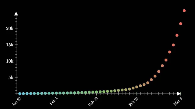
Exponential epidemic growth occurs when daily new cases are proportional to current cases, producing multiplication by a constant each day.
Briefing
Exponential growth in epidemics isn’t just a curve that looks steep—it’s a process where the number of new cases each day is proportional to the number of existing cases, so the daily change multiplies by a constant. In the COVID-19 data discussed here, daily case counts often behave like a factor of roughly 1.15 to 1.25 times the previous day’s total. That “multiply by a constant” mechanism is why small-looking daily increases can suddenly become enormous, and why comparing countries by raw case counts can mislead: a tenfold difference can correspond to only about a month of time if both are on the same exponential trajectory.
On a logarithmic scale, exponential growth appears as a straight line, making it easier to estimate the growth rate. Using the reported case data, the analysis suggests a pattern like “multiply by 10 every 16 days” on average, with a regression fit described as extremely close to the exponential model. The practical implication is stark: if the trend continued uninterrupted from the recording date (March 6), projections would reach about a million cases in 30 days, 10 million in 47 days, 100 million in 64 days, and 1 billion in 81 days. The key warning is that such straight-line extrapolations can’t last forever—real epidemics must eventually slow.
The slowdown isn’t arbitrary; it follows from the same math that creates exponential growth. In a simple model, each infected person exposes others at an average rate (E), and each exposure has a probability (p) of becoming a new infection. New cases scale like E·p·n, where n is the current number of cases—so growth accelerates as n grows. That acceleration can only stop if either E or p declines. Even in a worst-case “random mixing” scenario, growth eventually saturates because people being exposed are increasingly likely to already be infected; mathematically, this introduces a factor like (1 − fraction already infected), turning the early exponential into a logistic curve.
Logistic growth is exponential at first, then levels off as the epidemic approaches a limiting size. The transition point is the inflection point, where the number of new cases stops increasing and begins to fall. A practical way to detect this is the growth factor: the ratio of new cases on one day to new cases on the previous day. During the exponential phase, this ratio stays clearly above 1; when it approaches 1, the epidemic is nearing the inflection point. That creates a counterintuitive interpretation of “small” changes: a growth factor near 1 can mean the total cases will cap at roughly about twice the current level, while a growth factor still meaningfully above 1 implies orders of magnitude of growth may still be ahead.
Finally, the model’s assumptions can be relaxed. Real populations are clustered, not randomly mixed, but simulations with travel between clusters still produce similar exponential-inducing dynamics, often yielding a fractal-like structure where communities act like interacting units. Importantly, the two levers that reduce growth—lower exposure (E) and lower infection probability (p)—can change through behavior and policy: reduced gathering and travel, or improved hygiene like handwashing. The closing takeaway is both sobering and optimistic: if the growth rate drops, projections collapse dramatically; if it doesn’t, concern is warranted rather than complacency.
Cornell Notes
Epidemic exponential growth happens when daily new cases are proportional to the current number of cases, so each day multiplies by a roughly constant factor (about 1.15–1.25 in the COVID-19 example). On a logarithmic plot, that produces a straight line, letting analysts estimate rules like “multiply by 10 every 16 days.” Exponential growth can’t continue indefinitely because either exposure (E) or infection probability (p) must fall; even random mixing eventually saturates as more exposed people are already infected, producing a logistic curve. The inflection point is where the growth factor (new cases today ÷ new cases yesterday) approaches 1, signaling that new-case growth has stopped accelerating and totals will level off. Because growth is sensitive to the multiplication constant, small reductions in the daily factor can drastically shrink long-term projections.
Why does exponential growth feel “sudden” even when it’s consistent day to day?
How does the simple epidemic model produce exponential growth mathematically?
Why does a logarithmic y-axis make exponential growth look linear?
What marks the end of the exponential phase in the logistic model?
How can the growth factor be more informative than raw totals?
What real-world mechanisms can reduce exponential growth without relying on random mixing?
Review Questions
- If daily new cases multiply by a constant factor, what does that imply about how the growth factor behaves during the exponential phase?
- In the logistic model, what mathematical change prevents indefinite exponential growth, and how does that relate to the inflection point?
- Why can two countries with a 10× difference in case counts still be “close” in time if their growth factors match?
Key Points
- 1
Exponential epidemic growth occurs when daily new cases are proportional to current cases, producing multiplication by a constant each day.
- 2
In the COVID-19 example, daily case counts often align with a factor of about 1.15–1.25 times the previous day, making time-to-magnitude comparisons misleading.
- 3
Logarithmic plots turn exponential growth into a straight line, enabling estimates such as “multiply by 10 every 16 days.”
- 4
Exponential growth must end because either exposure (E) or infection probability (p) declines; saturation alone can force a logistic curve even under random mixing.
- 5
The inflection point is detected when the growth factor (new cases today ÷ new cases yesterday) approaches 1, signaling that new-case growth has stopped accelerating.
- 6
Small reductions in the multiplication constant can drastically shrink long-term projections, while unchanged growth rates justify continued concern.
- 7
Clustered populations can still show similar early dynamics if there is enough travel between communities, but behavior and hygiene can reduce E or p and slow spread.