Gradient descent, how neural networks learn | Deep Learning Chapter 2

Gradient descent is the engine behind neural-network learning: it repeatedly nudges thousands of adjustable weights and biases to reduce a single number called the cost. That cost measures how wrong the network’s outputs are across a large labeled training set—so “learning” becomes the practical task of finding a low point (a local minimum) in a very high-dimensional landscape. The method matters because it turns pattern recognition into an optimization problem that can be carried out with calculus, even when the model has around 13,000 parameters.

The setup starts with a digit classifier trained on MNIST-style images: each 28×28 grayscale image becomes 784 input values feeding a network with two hidden layers (16 neurons each) and 10 output neurons. For any image, the network produces 10 activations; the brightest output neuron is interpreted as the predicted digit. Before training, weights and biases are initialized randomly, producing outputs that look like noise and yield a high cost. The cost function is defined as the average, over all training examples, of the squared differences between the network’s output activations and the desired one-hot target (0 for most digits, 1 for the correct digit). Minimizing this average cost is meant to improve performance not only on the training set but also on new, unseen labeled images.

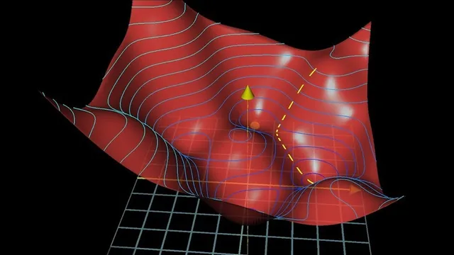
To reduce the cost, the process uses the gradient: in simple terms, the gradient points in the direction of steepest increase, so moving in the opposite direction decreases the cost fastest. For a function with many inputs—here, the entire vector of weights and biases—the negative gradient becomes a gigantic direction in parameter space. Each component of that gradient indicates both the sign (whether a particular weight should increase or decrease) and the relative magnitude (how much that weight change matters). With a small step size, repeated downhill moves shrink as the slope flattens near a minimum, helping avoid overshooting.

The computational work of obtaining these gradients efficiently is attributed to backpropagation, which will be unpacked next. A key conceptual requirement is that the cost surface should be smooth enough for small steps to reliably lead toward a minimum—one reason neural networks use continuously valued activations like sigmoid and ReLU rather than binary on/off units.

After training, the described “plain vanilla” architecture reaches about 96% accuracy on new MNIST images, with tuning of hidden-layer structure pushing performance toward roughly 98%. Yet the internal representations don’t match the earlier hope that early layers would clearly detect edges and later layers would assemble them into loops, lines, and digits. Visualizing the learned weights from the first to the second layer reveals patterns that are close to random, suggesting the network can find a workable local minimum without learning the intuitive feature hierarchy.

That tension—good accuracy versus unclear “understanding”—leads into modern research questions. One line of work shows that when labels are shuffled, a sufficiently large network can still memorize random mappings, achieving training accuracy comparable to structured training. Follow-up results at ICML suggest the optimization dynamics differ: accuracy drops more slowly on random labels, while structured labels allow faster descent into useful regions of the loss landscape. Related findings argue that the local minima reached by these networks can be “equal quality,” implying that structure in the dataset makes the right minima easier to find. The takeaway is that gradient descent is effective, but what it learns—and why it generalizes—depends on the geometry of the optimization landscape and the structure of the data.