Hilbert's Curve: Is infinite math useful?

Hilbert’s curve earns its keep by solving a practical mapping problem: turning a 2D image grid into a 1D sequence of frequencies in a way that stays stable as resolution increases. That stability matters because a naive “snake” ordering forces many pixel-to-frequency associations to jump around when the camera resolution changes—effectively resetting users’ learned intuition. A Hilbert-curve-style ordering, built from increasingly fine “pseudo-Hilbert” patterns, keeps each point on the frequency line moving less and less, so upgrades refine perception rather than break it.

The setup starts with a sound-to-sight thought experiment. Software takes low-resolution images (like 256×256 pixels), assigns each pixel a unique frequency, and plays louder tones for brighter pixels. If the mapping from pixel space (2D) to frequency space (1D) is arbitrary, the result is chaotic. The key design goal is continuity in a human sense: nearby frequencies should correspond to nearby locations in the image, so that small hearing errors don’t scatter the meaning across the grid.

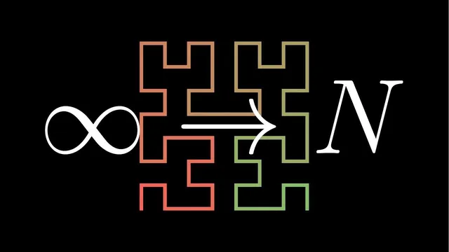
A “snake curve” achieves this by weaving through pixels row by row, but it has a fatal upgrade problem. When the grid doubles to 512×512, the same position along the frequency line can land in a very different place in the image—especially in the left-right direction—so users would have to relearn which tones correspond to which spatial features. The pseudo-Hilbert construction fixes that by recursively subdividing the square. At order one, the curve connects quadrant centers in a specific pattern. At order two, each quadrant contains a smaller order-one curve, with lower-left and lower-right pieces flipped to avoid awkward discontinuous jumps. Higher orders repeat the idea: subdivide, place smaller curves, flip where needed, and connect tip to tail.

For a 256×256 grid, the relevant order is eight; increasing resolution corresponds to increasing the order. The crucial property is that as the order grows, a fixed point along the curve approaches a specific location in the square rather than wandering erratically. In the finite, pixelated setting, pseudo-Hilbert curves approximate this behavior; in the continuous setting, the true Hilbert curve is defined as the limit of these approximations.

That infinite origin traces back to late-19th-century work on space-filling curves. After Peano’s first discovery in 1890, Hilbert produced a simpler curve in 1891. The goal was counterintuitive: construct a line-like object with zero area that nevertheless passes through every point of a 2D region. The modern definition hinges on continuity and on the convergence of the pseudo-Hilbert mappings for each input value between 0 and 1. Once the limit exists, the resulting function can be shown to be continuous and to fill the unit square.

The broader takeaway is philosophical but grounded in math: patterns developed to handle infinite objects often have finite analogs that become directly useful. Stability under refinement in the Hilbert construction mirrors the formal notion of limits, and similar correspondences appear elsewhere—such as how binary representations relate to infinite series of powers of 2. The practical lesson is to look beneath the surface of “infinite” results; the same machinery that proves them can often power finite tools people can actually use.