How (and why) to raise e to the power of a matrix | DE6

Matrix exponentiation—written as e^(At)—turns out to be a precise way to solve systems of differential equations where a state changes at a rate proportional to a matrix times the state. That matters because many real problems in science and engineering (and especially quantum mechanics) can be written in the form v'(t)=A v(t). Instead of guessing solutions, e^(At) packages the long-term evolution from time 0 to time t into a single matrix, so multiplying e^(At) by an initial condition vector produces the full trajectory.

The operation starts with a definition that looks like “plugging a matrix into the exponential,” but it’s not arbitrary. For real numbers, e^x is defined by its Taylor series; the matrix version uses the same infinite polynomial, term by term: exp(A)=I + A + A^2/2! + A^3/3! + … . This requires A to be square so that powers like A^2, A^3, and so on are well-defined via repeated matrix multiplication. Adding matrices works term-by-term as well, so the Taylor-series construction makes sense as a formal infinite sum—at least in cases where it converges.

A concrete example makes the definition feel less like notation abuse. Take the 2×2 matrix with −π and π on the off-diagonal: [[0, −π],[π, 0]]. When its Taylor-series exponential is computed, the sum approaches −I, the negative identity matrix. That result isn’t a coincidence: it’s the matrix analogue of Euler’s identity, and it reflects what happens when the underlying matrix represents a 90-degree rotation. Exponentiating a rotation operator for time t generates the rotation by angle t; after π units of time, a 90-degree-per-unit-time rotation becomes a 180-degree flip, which is exactly multiplication by −1.

The “why” becomes clearer through differential equations. The Romeo-and-Juliet relationship model encodes two coupled rates of change: one person’s feelings increase when the other’s decrease, and vice versa. Writing the pair (x(t), y(t)) as a vector v(t) turns the system into v'(t)=M v(t), where M is a specific 2×2 matrix. Geometrically, M acts like a 90-degree rotation, so the velocity vector is always perpendicular to the position vector. That constraint forces circular motion at a constant angular speed, giving explicit solutions that match what e^(Mt) produces.

The same framework scales up. In one dimension, x'(t)=r x(t) has solutions x(t)=x0 e^(rt), showing that the exponential acts on an initial condition. In higher dimensions, the exponential becomes a matrix-valued operator: e^(At) plays the role of “the thing that turns initial data into the evolving state.” A quick calculus check supports this: differentiating the Taylor-series expression for e^(At) yields A times the original expression, so it satisfies v'(t)=A v(t) (with convergence details handled separately).

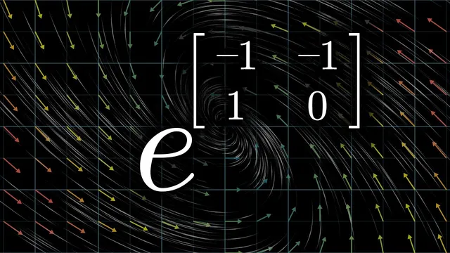
Finally, the discussion connects the idea to quantum mechanics. Schrödinger’s equation has the same structural core—time evolution governed by a matrix acting on a state vector—but the matrix includes the imaginary unit i, which enforces oscillatory behavior. More generally, the evolution can be visualized with a vector field where each point v has velocity Mv; flowing along that field for time t produces the transformation encoded by e^(Mt).