Integration and the fundamental theorem of calculus | Chapter 8, Essence of calculus

Integration is the inverse of differentiation in a precise sense: the accumulated area under a velocity curve produces a distance function whose derivative at any time equals the original velocity. That link matters because it turns “add up infinitely many tiny contributions” into a computation that only needs two evaluations—at the upper and lower bounds—once an antiderivative is found.

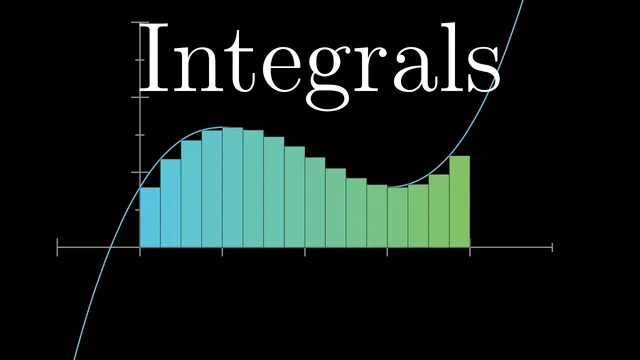
The discussion begins with a car problem. With no view outside the window, the only information available is the speedometer reading over time. If velocity were constant, distance would be velocity times elapsed time—an area rectangle on a graph where time is horizontal and velocity is vertical. Real motion is harder because velocity changes continuously, so the approach is to approximate the changing velocity by treating it as constant over many short intervals. On each small interval of length dt, the car’s distance contribution is approximated by “(velocity at the left endpoint) × dt,” which corresponds to the area of a thin rectangle. Summing these rectangle areas across the time range gives an approximation to total distance.

As dt shrinks toward zero, the rectangle sum converges to the exact area under the velocity curve. This limiting area is written as an integral of v(t) over time. The key intuition is that the integral is built from every input between the bounds—yet the final computation can be expressed in a surprisingly economical way.

To connect area to derivatives, the upper bound is treated as a variable capital T. Define a distance function s(T) as the area under the velocity graph from 0 to T. A small increase in T by dt adds a thin sliver of area ds. For sufficiently small dt, that sliver is essentially a rectangle whose height is v(T) and width is dt, so ds/dt equals v(T). In other words, differentiating the “area-so-far” function recovers the original function that generated the area.

Once this relationship is accepted, the fundamental theorem of calculus follows. If v(t) is the integrand, then finding a function F(t) whose derivative is v(t) (an antiderivative) allows the integral to be computed as F(upper bound) minus F(lower bound). There are infinitely many antiderivatives because adding a constant doesn’t change derivatives, but the subtraction of the lower-bound value cancels that ambiguity automatically.

A concrete example uses v(t)=t(8−t)=8t−t^2. An antiderivative is 4t^2−(1/3)t^3, so the distance from time 1 to 7 comes from evaluating that expression at 7 and subtracting its value at 1.

Finally, the treatment emphasizes signed area. If velocity becomes negative (the car moves backward), the corresponding rectangles lie below the horizontal axis, contributing negative distance change. Integrals therefore measure signed area between the graph and the axis, not just geometric area in the everyday sense. The result is a unified method for turning accumulation problems—like distance from velocity—into derivative/antiderivative relationships that can be computed efficiently.