Lecture 11B: Monitoring ML Models (Full Stack Deep Learning - Spring 2021)

Monitoring deployed machine learning models is about catching silent performance decay—often driven by changes in data, user behavior, or sampling artifacts—before it turns into revenue loss. After deployment, model quality rarely stays fixed: input distributions shift (data drift), the relationship between inputs and outcomes changes (model or concept drift), and the way training data was sampled can leave blind spots (domain shift/long-tail gaps). The practical takeaway is that “ship and forget” fails because ML systems degrade through subtle, hard-to-detect changes rather than loud crashes.

The lecture frames drift through three probability-level failure modes. First, p(x) can change: upstream pipelines may redefine features or introduce bugs (e.g., a feature suddenly becoming all -1), malicious users can feed adversarial inputs, new regions or new user demographics can alter the input mix. Second, p(y|x) can change, often because user behavior adapts to the model—especially in recommenders, where clicks reshape future preferences. Third, sampling artifacts can matter: long-tail events that occur rarely but are costly when wrong may be underrepresented, and bias in sampling can systematically exclude critical cases.

Drift isn’t just theoretical; it shows up in production. During the pandemic, widespread distribution shifts caused many models to drift, leading to unexpected behavior. In one e-commerce-style case, a retraining pipeline bug repeatedly served the same recommendations, driving churn and costing millions over a month or two before detection. These examples motivate a structured monitoring plan.

The lecture lays out what to monitor using four signal types, ordered by how directly they reflect model performance and how hard they are to obtain. The most informative is ground-truth model performance, but labels are often delayed or expensive. Business metrics (click-through rate, engagement) are easier to measure but can be confounded by many factors unrelated to accuracy. Input and prediction distributions help detect drift without labels, though measuring them well takes care. System health metrics (GPU utilization, latency) are straightforward but only catch coarse failures like crashes or memory leaks.

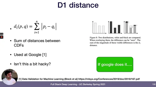
To measure change, monitoring systems compare a “reference” distribution to a “current” window. A pragmatic default is using training/evaluation data as the reference. Windowing can be fixed (e.g., last day) or sliding (e.g., last hour), and there’s a special case where window size equals one, leading toward outlier detection. For distance metrics, rule-based data quality checks (ranges, missingness, ordering constraints) are recommended as a strong first layer because they catch many issues and are easier to operationalize. Statistical distances exist—KS statistic is favored for interpretability, while KL divergence is discouraged due to tail sensitivity, asymmetry, and numerical pitfalls.

Deciding whether a detected change is “bad” remains less settled. Statistical tests can produce tiny p-values with large datasets even for negligible shifts, so teams often rely on thresholds, anomaly detection, and manual rule-setting. Tooling is emerging across three categories: system monitoring (e.g., CloudWatch), data quality frameworks (e.g., Great Expectations), and ML monitoring platforms (e.g., Arize, Arthur, Fiddler).

Finally, monitoring should be integrated into the broader ML lifecycle, not bolted on. The lecture argues for an “evaluation store” that ties monitoring to offline evaluation and training—helping close the data flywheel by guiding what to label, how to oversample low-performing regions, and when retraining is worth the compute and data cost. The field still lacks mature research on linking drift scores to actual performance impact, leaving major open problems for reliable ML in the real world.