Lecture 2A: Convolutional Neural Networks (Full Stack Deep Learning - Spring 2021)
Based on The Full Stack's video on YouTube. If you like this content, support the original creators by watching, liking and subscribing to their content.
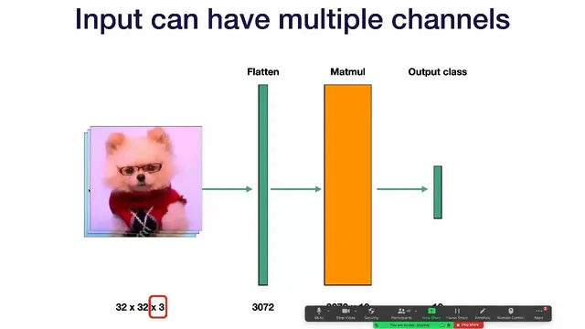
Fully connected image models flatten pixels into a large vector, causing weight counts to grow rapidly with image resolution.
Briefing
Convolutional neural networks gained their edge in computer vision by replacing the “flatten an image and learn a giant matrix” approach with a sliding, weight-sharing operation that scales far better as images get larger. Fully connected networks treat every pixel as a distinct input feature, so the number of learnable weights grows rapidly with image size: a 32×32 grayscale image flattens to 1024 values, but moving to 64×64 multiplies the input dimensionality by four, and 128×128 multiplies it by sixteen—ballooning the parameter count. Convnets also address a second weakness: fully connected models are not naturally invariant to translations. If an object shifts a few pixels, the fully connected layer effectively “looks at” different pixel positions, so the model’s outputs can change unless translation robustness is engineered via augmentation.
A convolutional filter fixes both issues by operating on local patches and reusing the same learned weights across the image. Instead of multiplying a whole-image vector by a massive matrix, a conv layer extracts a small window—commonly 5×5—flattens it, and computes a dot product with a learned weight vector to produce one output value for that patch. Sliding the window across height and width yields an output map with one value per patch location. Historically, carefully chosen convolution kernels could perform interpretable image processing like blurring; modern convnets learn those weights directly from data.
The core operation extends naturally to color images and multiple feature maps. For RGB inputs shaped 32×32×3, a 5×5×3 patch contains 75 values, so each filter learns 75 weights. Applying multiple filters produces multiple channels in the output tensor: for example, 10 filters can turn a 28×28×3 input into a 28×28×10 output. Crucially, the output has the same three-dimensional tensor structure as the input, enabling stacking: one convolutional layer’s output can feed the next. Because each convolution is linear, convnets typically insert a nonlinearity (often ReLU) after each convolution to increase expressiveness.
Two practical knobs control how the filter moves and how tensor sizes change. Stride determines the step size of the sliding window; larger strides skip positions and downsample the feature map. Padding adds a border around the input (often zeros) so the filter can still be applied near edges; “same” padding is designed to keep output spatial dimensions equal to input, while “valid” uses no padding. Output sizes follow standard arithmetic based on input size, filter size, stride, and padding.
Beyond basic convolution, the lecture highlights operations that shape what the network can “see” and how it compresses information. Stacking convolutions increases the receptive field: two 3×3 layers can match the spatial coverage of a single 5×5, often with better empirical performance due to added nonlinearity. Dilated convolutions expand receptive field without increasing parameters by skipping pixels inside the kernel footprint. To reduce spatial dimensions, pooling—especially 2×2 max pooling—summarizes local regions by taking max (or sometimes average). A 1×1 convolution reduces channel depth while mixing information across channels at each spatial location.
As a baseline architecture, the lecture describes the classic LeNet-style pattern: repeated blocks of convolution + nonlinearity, followed by pooling, then fully connected layers and a softmax output. The discussion also clarifies training pragmatics, such as placing activations between fully connected layers but avoiding a nonlinearity after the final fully connected layer when the loss function expects raw logits.
Cornell Notes
Convolutional neural networks replace fully connected image processing with local, sliding filters that reuse the same weights across the image. This avoids the rapid parameter growth of fully connected layers and improves translation robustness because the same detector responds wherever the pattern appears. Convnets stack convolution layers (with nonlinearities) to build richer features, while stride and padding control downsampling and output sizes. Receptive field expands through stacking or dilated convolutions, and pooling or 1×1 convolutions reduce spatial size or channel count. A LeNet-style architecture—conv + activation + pooling repeated, then fully connected layers and softmax—serves as a classic baseline.
Why do fully connected networks scale poorly for images, and how does convolution address that?
How does a convolutional filter produce an output map from an image?
What roles do stride and padding play in convolutional layers?
How can receptive field grow without using larger kernels?
What are pooling and 1×1 convolutions used for?
What is the LeNet-style convolutional architecture pattern described here?
Review Questions
- How does parameter count in a fully connected image model change as image resolution increases, and why does weight sharing in convolution prevent the same scaling problem?
- Given a convolution with a certain filter size, stride, and padding, what determines the output spatial dimensions, and how do “same” and “valid” differ?
- Why might two stacked 3×3 convolutions outperform a single 5×5 convolution even when they cover the same receptive field?
Key Points
- 1
Fully connected image models flatten pixels into a large vector, causing weight counts to grow rapidly with image resolution.
- 2
Convolutional filters operate on local patches and reuse the same weights across spatial locations, improving both scalability and translation robustness.
- 3
Stacking convolution layers (with nonlinearities) builds increasingly complex features because each layer’s output retains a tensor structure suitable for further convolutions.
- 4
Stride down-samples by skipping filter positions, while padding (often zeros) prevents edge information from being discarded; “same” padding targets equal input/output spatial sizes.
- 5
Receptive field expands through stacking or dilated convolutions; dilations enlarge coverage without adding parameters by skipping pixels within the kernel footprint.
- 6
Pooling (commonly 2×2 max pooling) reduces spatial dimensions, while 1×1 convolutions reduce channel depth by mixing information at each pixel location.
- 7
A LeNet-style baseline alternates conv + activation and pooling blocks, then uses fully connected layers and softmax for classification.