Lecture 2B: Computer Vision Applications (Full Stack Deep Learning

TL;DR

ImageNet’s shift from shallow models to deep networks accelerated after AlexNet cut top-5 error dramatically using dropout, heavy augmentation, and multi-GPU training.

Briefing Cornell Notes

Briefing

Computer vision deep learning has advanced largely by swapping in better image-recognition backbones—then reusing those same building blocks for localization, detection, segmentation, and even 3D and adversarial robustness. The through-line is that architectures trained for ImageNet classification (especially AlexNet, VGG, GoogLeNet/Inception, and ResNet) became a toolbox: convolutional feature extractors plus training tricks, visualization methods, and efficient heads for different output formats.

The ImageNet Large Scale Visual Recognition Challenge, introduced in 2010, set the stage with 1,000 categories and over a million training images. Early winners relied on shallow methods like SVMs, with error rates around 25%. In 2012, AlexNet—an eight-layer deep network—cut the error rate to about 16%, triggering the deep-learning shift. AlexNet’s gains came from several practical engineering choices: dropout to randomly zero weights during training, heavy data augmentation (horizontal flips, rotations, scaling, and random crops), and multi-GPU distributed training because the model fit only by splitting it across two GPUs. Architecturally, it used a familiar conv/pooling stack (e.g., 11×11 then 5×5 then 3×3 convolutions) followed by fully connected layers.

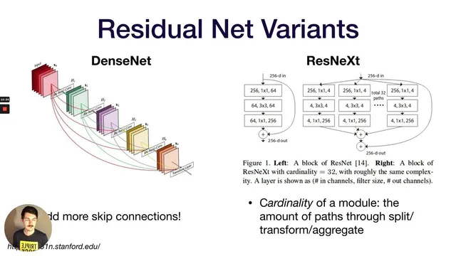
Subsequent years refined the same core idea. VGG pushed depth while standardizing on 3×3 convolutions and 2×2 max pooling, arguing that stacking multiple 3×3 layers yields the same receptive field as a larger kernel (like 9×9) with fewer parameters. GoogLeNet (Inception) reduced parameter counts by removing fully connected layers and using “inception modules” that process the same input through multiple convolutional paths (1×1, 3×3, stacked 3×3, and pooling) and concatenate the results. It also added auxiliary classifier outputs mid-network to improve gradient flow. ResNet then addressed a key failure mode of simply going deeper: vanishing gradients. Residual connections add skip paths so gradients can propagate through identity shortcuts, enabling very deep models (152 layers) and achieving top-5 error lower than human performance on ImageNet.

Beyond classification, the lecture mapped how to turn a classifier into other vision systems. Localization can be done by adding bounding-box coordinate outputs (x1, y1, x2, y2), but detection must handle an unknown number of objects. One approach is “sliding-window” classification over many overlapping regions, made efficient by converting fully connected layers into 1×1 convolutions and then using non-maximum suppression to prune overlapping boxes based on detection scores. This lineage includes YOLO-style “look once” detectors that place a grid over the image and predict class probabilities and bounding boxes per cell, then apply non-maximum suppression. Another approach uses region proposals: R-CNN, Faster R-CNN (with a region proposal network), and Mask R-CNN, which adds a segmentation head for instance masks.

Segmentation generalizes further into fully convolutional networks (U-Net style ideas), where downsampling and upsampling reconstruct pixel-level masks using techniques like unpooling, transpose convolutions, and dilated convolutions. The same multi-head pattern extends to 3D via Mesh R-CNN, which predicts voxel/mesh outputs using datasets like ShapeNet. The lecture also highlighted why these systems can be brittle: adversarial attacks exploit how networks behave off the data manifold, turning imperceptible or even physically realizable perturbations into high-confidence misclassifications. Finally, it broadened the vision toolbox to style transfer, GANs, and practical learning resources like Papers with Code for tracking benchmarks and state-of-the-art methods.

Cornell Notes

ImageNet classification breakthroughs—AlexNet, VGG, GoogLeNet/Inception, and especially ResNet—built the core feature-extraction toolbox for modern computer vision. AlexNet’s jump came from dropout, heavy augmentation, and multi-GPU training; VGG standardized on 3×3 convolutions to expand receptive field efficiently; GoogLeNet used inception modules and auxiliary classifiers to cut parameters and improve gradients; ResNet added residual skip connections to prevent degradation as depth increases. Once a strong classifier exists, the same convolutional backbone can be adapted for localization, detection, and segmentation by changing the output heads and adding post-processing like non-maximum suppression. The lecture also extended the pattern to instance segmentation (Mask R-CNN), dense prediction (fully convolutional/U-Net style ideas), 3D reconstruction (Mesh R-CNN), and robustness challenges like adversarial attacks.

Why did AlexNet’s 2012 results matter so much for computer vision?

AlexNet’s deep architecture reduced ImageNet error from roughly ~25% (shallow methods) to about 16% in 2012, which shifted the field toward deep networks. It combined dropout (randomly zeroing weights during training), heavy data augmentation (flips, rotations, scaled crops), and multi-GPU distributed training to fit the model given limited GPU memory. Its conv/pooling stack (e.g., 11×11 then 5×5 then 3×3 convolutions with max pooling) produced hierarchical features that later layers could interpret as parts of objects.

What efficiency idea did VGG introduce with 3×3 convolutions?

VGG argued that stacking multiple 3×3 convolutions can match the receptive field of a larger kernel (like a 9×9 convolution) while using fewer parameters. It also used 2×2 max pooling and increased channel depth across layers (e.g., early layers with ~64 channels, later layers with ~512). The lecture noted that memory costs often rise in early conv layers due to large intermediate activations, while parameter-heavy fully connected layers dominate weight count.

How did GoogLeNet’s inception modules reduce parameters while improving training signals?

GoogLeNet/Inception replaced single-path processing with parallel branches inside an inception module: 1×1 convolutions, 3×3 convolutions (often stacked), and pooling, then concatenation of branch outputs. A key trick was using 1×1 convolutions first to reduce channel dimensionality before expensive spatial convolutions, leveraging the idea that cross-channel correlations and spatial correlations can be treated separately. It also added auxiliary classifier heads mid-network so gradients reached earlier layers, helping optimization.

What problem did ResNet solve, and how do residual connections work?

ResNet targeted the observation that making networks deeper doesn’t always improve accuracy because gradients can vanish or training can degrade. Residual connections add skip paths that let the gradient flow through an identity route. The computation is framed as y = h(x) + x, where h(x) is the learned transformation and x is the shortcut, so the network effectively learns a residual correction rather than an entirely new mapping.

How do detection systems turn a classifier into bounding boxes and multiple objects?

Localization can be done by adding bounding-box coordinate outputs (x1, y1, x2, y2) to a classifier, but detection must handle an unknown number of objects. One strategy is to run a sliding-window classifier over many overlapping regions efficiently by converting fully connected layers into 1×1 convolutions, producing many candidate boxes. Non-maximum suppression then keeps the highest-scoring boxes and removes others with high overlap. YOLO-style detectors go further by predicting boxes and class probabilities from a fixed grid in a single pass, then applying non-maximum suppression.

Why are adversarial attacks possible even when models perform well on normal data?

The lecture described a manifold intuition: networks learn a complex mapping from images to categories/segmentations that works well on the training-data manifold. Small perturbations can push inputs off that manifold, causing confident misclassifications. An example described adding noise that looks like a panda to humans but triggers a different class with high confidence (e.g., “nematode”). It also noted physical-world attacks—like altering printed patterns on road signs—to mislead systems such as those used in self-driving contexts.

Review Questions

Which architectural changes in AlexNet, VGG, GoogLeNet, and ResNet were aimed at accuracy gains, and which were aimed at training stability or parameter efficiency?
Explain how non-maximum suppression and intersection-over-union (IoU) relate to evaluating detection quality.
Pick one detection family (YOLO-style or R-CNN-style) and describe how it generates candidate boxes and then filters them.

Key Points

1
ImageNet’s shift from shallow models to deep networks accelerated after AlexNet cut top-5 error dramatically using dropout, heavy augmentation, and multi-GPU training.
2
VGG’s 3×3 convolution stacking achieves the same receptive field as larger kernels with fewer parameters, trading compute patterns for parameter efficiency.
3
GoogLeNet’s inception modules reduce parameter count by using 1×1 convolutions for channel reduction and parallel multi-scale feature extraction, while auxiliary classifiers improve gradient flow.
4
ResNet’s residual skip connections prevent degradation in very deep networks by preserving gradient pathways through identity shortcuts.
5
Detection systems adapt classification backbones by predicting bounding boxes and then using non-maximum suppression to remove redundant overlapping detections.
6
Segmentation extends classification into dense prediction via fully convolutional encoder–decoder designs and upsampling methods like transpose convolutions or unpooling.
7
Adversarial attacks exploit how models behave off the learned data manifold, enabling high-confidence errors from subtle or even physical perturbations.

Highlights

AlexNet’s 2012 ImageNet breakthrough combined dropout, aggressive augmentation, and distributed training to make deep learning practical at the time.

VGG’s “3×3 everywhere” design showed how stacking small kernels can replicate larger receptive fields with fewer parameters.

ResNet’s identity shortcuts turned depth from a liability into an advantage by stabilizing gradient flow.

YOLO-style detectors generate many candidate boxes in one pass using a grid, then rely on non-maximum suppression for final predictions.

Adversarial examples can make an image look unchanged to humans while driving a network to a different class with extreme confidence.

Topics

ImageNet Classification
Convolutional Backbones
Object Detection
Instance Segmentation
Adversarial Attacks

Mentioned

IoU
SVM
GPU
YOLO
SSD
RCNN
U-Net
GAN
R-CNN
Faster R-CNN
Mask R-CNN
COCO

Lecture 2B: Computer Vision Applications (Full Stack Deep Learning - Spring 2021)