Lecture 3: Recurrent Neural Networks (Full Stack Deep Learning - Spring 2021)
Based on The Full Stack's video on YouTube. If you like this content, support the original creators by watching, liking and subscribing to their content.
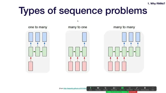
Sequence modeling tasks can be categorized by whether inputs and outputs are single values or sequences, including many-to-one, one-to-many, and many-to-many settings.
Briefing
Recurrent neural networks (RNNs) were built to handle sequence data efficiently by reusing the same weights across time and carrying information forward in a hidden state—an approach meant to exploit patterns that repeat over a sequence rather than treating every position as unrelated. The lecture frames sequence modeling as a set of problem types—time-series forecasting, translation, speech, image captioning, and question answering—then argues that feedforward networks struggle with variable-length sequences and become data-inefficient when they must learn position-specific mappings for repeated patterns.
In the core RNN setup, each time step takes the current input x_t and the previous hidden state h_{t-1}, computes a new hidden state h_t, and produces an output y_t. The hidden-state update is described as two matrix multiplications—one for h_{t-1} and one for x_t—summed and passed through an activation function (the basic form uses tanh). This weight sharing across time replaces the “single massive matrix” approach and makes the architecture naturally suited to sequences of varying length. For tasks where only one output is needed at the end (many-to-one), the last hidden state is fed into a classifier; for tasks where an output sequence must be generated from a single input (one-to-many), an encoder-decoder pattern is used: an encoder compresses the input into an initial state, and a decoder generates outputs step-by-step.
The lecture then zooms in on why vanilla RNNs break down on long sequences: backpropagation through time multiplies gradients across many steps, and with common activations like sigmoid and tanh, derivatives shrink toward zero, leading to vanishing gradients. The result is that long-term dependencies—like remembering a character name introduced early in a long sentence—get lost. LSTMs (Long Short-Term Memory networks) address this by adding a separate cell state plus gating mechanisms. A forget gate decides what to remove from the cell state, an input gate controls what new information to add, and the output computation uses a gated version of the cell state to produce the next hidden state. The lecture notes that GRUs and other variants exist, and cites empirical findings suggesting regular LSTMs are hard to beat across datasets, while GRUs can sometimes train more easily or perform slightly better.
Machine translation serves as a case study for how RNN encoder-decoder systems were made practical. The baseline idea—encode the source sentence with an RNN and initialize the decoder with the final encoder state—creates an information bottleneck for long sentences. Improvements include stacking LSTM layers (with residual connections to make deeper stacks trainable), adding attention so the decoder can access a weighted summary of all encoder hidden states instead of only the last one, and using bidirectionality so the encoder reads the sentence in both forward and backward directions. Attention is described via relevance weights over encoder states, producing attention maps that show which source words influence each target word.
Finally, the lecture introduces CTC loss (Connectionist Temporal Classification) for sequence tasks with misalignment, using handwriting recognition as the motivating example. CTC allows the model to emit characters or a special blank (epsilon) token at each time step, then merges repeated characters and removes blanks to produce the final transcription—handling cases where input and output lengths differ. The lecture closes by weighing RNN trade-offs: flexible architectures and strong historical performance versus slower, less parallelizable training, which helped open the door for transformers. It previews non-recurrent alternatives such as WaveNet-style convolutional sequence models, using causal and dilated convolutions to capture long-range context while enabling parallel training, at the cost of more expensive inference.
Cornell Notes
Sequence problems come in many-to-one, one-to-many, and many-to-many forms, and RNNs handle them by carrying a hidden state forward while reusing the same weights at every time step. Vanilla RNNs struggle with long-term dependencies because backpropagation through time multiplies gradients across many steps, causing vanishing gradients (or sometimes exploding gradients). LSTMs fix this with a cell state and gates—forget, input, and output—that regulate what information persists and what gets updated. For machine translation, encoder-decoder RNNs were improved with stacked LSTMs, residual connections, attention (so the decoder can use all encoder states via relevance weights), and bidirectional encoding. When alignment between input and output is unclear, CTC loss supports transcription by emitting characters or blanks and then merging repeats while removing blanks.
Why do feedforward networks become awkward for sequence tasks with variable length and repeating patterns?
How does a basic RNN compute outputs across time, and what makes it more efficient than a single flattened matrix?
What exactly breaks down in vanilla RNNs on long sequences, and how do LSTMs address it?
Why did early RNN encoder-decoder translation systems need attention?
How does CTC loss handle misalignment between input time steps and output characters?
What trade-off does WaveNet-style convolutional sequence modeling make compared with RNNs?
Review Questions
- How does backpropagation through time lead to vanishing gradients in vanilla RNNs, and why do tanh/sigmoid derivatives matter?
- In an encoder-decoder translation system, what bottleneck does attention remove, and how do relevance weights determine what the decoder uses?
- During CTC decoding, what role do blank (epsilon) tokens play in producing repeated characters correctly?
Key Points
- 1
Sequence modeling tasks can be categorized by whether inputs and outputs are single values or sequences, including many-to-one, one-to-many, and many-to-many settings.
- 2
Vanilla RNNs reuse weights across time by updating a hidden state from (x_t, h_{t-1}), but they struggle with long-term dependencies due to vanishing gradients.
- 3
LSTMs add a cell state and gating (forget, input, output) to regulate information flow and preserve long-range context.
- 4
Early neural machine translation with RNN encoder-decoders improved performance using stacked LSTMs with residual connections, attention over all encoder states, and bidirectional encoding.
- 5
Attention replaces the fixed-size encoder bottleneck by computing relevance weights and forming weighted sums of encoder hidden states, often visualized as attention maps.
- 6
CTC loss supports sequence tasks with unknown alignment by emitting characters or blanks at each time step and then merging repeats while removing blanks.
- 7
RNNs are flexible but slower to train because they require sequential computation; convolutional alternatives like causal/dilated models improve training parallelism but can make inference more costly.