Lecture 4: Transfer Learning and Transformers (Full Stack Deep Learning - Spring 2021)
Based on The Full Stack's video on YouTube. If you like this content, support the original creators by watching, liking and subscribing to their content.
Transfer learning reuses large pre-trained feature extractors and fine-tunes only task-specific layers to avoid overfitting on small labeled datasets.
Briefing
Transfer learning is the bridge that lets large, pre-trained neural networks work on small, task-specific datasets—first in computer vision, then in language. In the bird-classification example, a model like ResNet50 trained on ImageNet (about a million images) would overfit if trained from scratch on only 10,000 labeled bird images. The practical fix is to reuse the ImageNet-trained layers and fine-tune only the final parts: keep the convolutional “feature extractor” weights, freeze them so gradients aren’t stored, and train a small classifier head on the new data. Frameworks such as PyTorch (via torchvision) and TensorFlow make this workflow straightforward through model zoos and pre-trained weights.
That same reuse idea becomes the core of modern NLP, but it starts with a different representation problem: words must become vectors. One-hot encoding works but scales poorly because vocabulary size directly inflates sparse, high-dimensional inputs and breaks intuition about similarity (e.g., “run” and “running” end up equally distant from unrelated words). Embeddings solve this by mapping each word to a dense vector via an embedding matrix, which can be learned during a task or—more powerfully—pre-trained on large text corpora. A classic pre-training route is next-word prediction: slide a window over text, train a model to predict the next token with cross-entropy, and optionally use skip-gram-style objectives that treat nearby words as positives and distant words as negatives. The payoff is that embedding vectors support meaningful “vector math,” capturing relationships like tense changes (walking→walked) and analogies such as country–capital patterns.
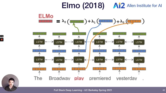
Around 2017, NLP’s “ImageNet moment” arrives with deeper pre-training beyond shallow embeddings. Instead of only using embeddings as the first layer, models pre-train richer stacks—often using bidirectional LSTMs—to capture context that embeddings alone can’t. ELMo (2018) uses a bidirectional stacked LSTM to improve performance on benchmarks like SQuAD (question answering), SNLI (natural language inference), and GLUE (a suite of tasks including entailment, paraphrase, and sentiment). ULMFiT follows a similar spirit with bidirectional LSTMs and pre-trained representations, and by 2018–2019 these pre-trained language models become standard in model gardens.
Transformers then take over as the foundational architecture, introduced by “Attention Is All You Need” (2017). Transformers replace recurrence with attention: each token is transformed into Query, Key, and Value vectors, and attention computes weighted sums of other tokens to build contextual representations. Multi-head attention learns multiple sets of these projections in parallel, while layer normalization stabilizes training by resetting mean/variance between layers. Positional embeddings inject order information, and causal masking lets GPT-style models predict the next token using only past context.
The lecture traces major transformer families and scaling trends: GPT models are generative and unidirectional (causal masking), BERT-style models are bidirectional (masked-token prediction), and T5 reframes tasks by encoding both inputs and outputs as text strings, achieving strong results on GLUE and SuperGLUE with an encoder–decoder setup. Model sizes balloon—from GPT-2’s 1.5B parameters to GPT-3’s ~175B—driving large accuracy gains with architecture largely unchanged, a pattern framed as the “bitter lesson.” But compute costs and misuse risks also rise: GPT-3 weights were not released publicly due to societal concerns, and the lecture highlights both impressive capabilities (including code generation and even text-to-image via DALL·E) and failure modes like biased or nonsensical outputs. Finally, it points to a countertrend for limited budgets: distillation (e.g., DistilBERT), which trains a smaller model to retain most performance of a larger one, and to tooling ecosystems like Hugging Face Transformers that make pre-trained models widely usable.
Cornell Notes
The lecture connects transfer learning in vision to the rise of pre-trained language models in NLP. Instead of training from scratch on small datasets, models reuse large pre-trained representations: freeze most layers, then fine-tune a small task-specific head. In language, dense embeddings replace sparse one-hot vectors, and pre-training (e.g., next-word prediction) yields vectors that support useful relationships. Around 2017–2018, deeper pre-trained models like ELMo and ULMFiT improved major benchmarks, leading to the “ImageNet moment” for NLP. Transformers then became the dominant architecture by using attention (queries/keys/values), positional embeddings, layer normalization, and masking; GPT, BERT, and T5 differ mainly in directionality and training objectives.
Why does transfer learning help when labeled data is scarce, and what exactly gets frozen?
What problem with one-hot encoding motivates word embeddings?
How does next-word prediction pre-training create useful embeddings?
What makes transformers different from earlier sequence models like LSTMs?
How do GPT, BERT, and T5 differ in training objective and information flow?
Why do model sizes matter so much, and what countermeasures exist?
Review Questions
- How does freezing pre-trained layers during fine-tuning prevent overfitting on small datasets, and which parts are typically trained instead?
- Describe the roles of Query, Key, and Value in self-attention and explain how masking changes what information a model can use.
- Compare GPT, BERT, and T5 in terms of directionality (causal vs bidirectional) and how their training objectives shape their outputs.
Key Points
- 1
Transfer learning reuses large pre-trained feature extractors and fine-tunes only task-specific layers to avoid overfitting on small labeled datasets.
- 2
Freezing pre-trained weights (e.g., via eval mode in PyTorch) prevents gradient updates, so only newly added classifier layers learn from the target data.
- 3
One-hot encoding scales poorly and produces sparse, high-dimensional vectors that don’t reflect word similarity; dense embeddings address both issues.
- 4
Pre-training language models on large corpora using objectives like next-word prediction yields embedding spaces that support useful linguistic relationships via vector math.
- 5
Transformers replace recurrence with attention using Query/Key/Value projections, multi-head attention, positional embeddings, layer normalization, and masking.
- 6
GPT, BERT, and T5 mainly differ in directionality and training setup: causal next-token generation, bidirectional masked prediction, and text-to-text encoder–decoder framing, respectively.
- 7
Scaling parameter counts has driven major accuracy gains, but compute costs and misuse risks have led to access restrictions and to smaller-model alternatives like knowledge distillation.