Lecture 6: Infrastructure & Tooling (Full Stack Deep Learning - Spring 2021)
Based on The Full Stack's video on YouTube. If you like this content, support the original creators by watching, liking and subscribing to their content.
Continuous model improvement requires a repeatable data-to-deployment feedback loop, including monitoring and dataset updates from production.
Briefing
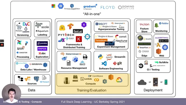
Deep learning progress depends less on model code than on the surrounding “infrastructure and tooling” that turns raw data into continuously improving systems. The practical dream—ship a scalable model, generate new production data, retrain, and deploy again—only works if teams can repeatedly collect, clean, label, version, and monitor data; run and debug training experiments; and then keep deployed models healthy by feeding back new examples. That loop is the real engineering challenge, and it’s why so much effort goes into building reliable pipelines rather than just writing neural networks.
A useful way to organize this work splits it into three buckets: data, training/evaluation, and deployment (with data feedback spanning all three). Data engineering includes sources like logs, databases, files, and images, plus storage layers such as data lakes and warehouses (examples named include Databricks, Snowflake, BigQuery, and Redshift). Processing and transformation rely on tools like Airflow, Apache Spark, and Dagster, with exploration and transformation often done via pandas and SQL-oriented workflows using dbt. Many datasets also require labeling, and the outputs must be versioned into reproducible artifacts.
Training and evaluation then demand both general software engineering and deep-learning-specific tooling. Python dominates because of its ecosystem, and the workflow is shaped by editors and IDEs such as Visual Studio Code (with features like version control, diffs, inline documentation, and remote notebook support). Static analysis and type hints—via linters and tools like PyLint—help codify style rules and catch bugs early. Notebooks (Jupyter) remain common for prototyping, but they’re criticized for versioning difficulty, fragile execution order, and poor support for testing and distributed jobs; alternatives like Streamlit are positioned for interactive “applets” built directly from Python.
On the compute side, the lecture frames deep learning as a scaling problem: results increasingly consume more compute, pushing teams toward multi-GPU and multi-node training. GPU choice matters—especially memory capacity and mixed-precision support via NVIDIA tensor cores—so architectures and models (Kepler, Pascal, Volta, Turing, Ampere) are discussed alongside practical options like V100 and A100 in the cloud. The tradeoff between on-prem and cloud is treated as a cost-versus-speed decision, with spot/preemptible instances offered as a way to run many experiments faster when time is critical.
To manage compute efficiently, resource schedulers such as Slurm are recommended for allocating GPUs and dependencies across teams. For packaging environments, Docker and Kubernetes (including Kubeflow) are mentioned, alongside “all-in-one” platforms that reduce setup overhead. Training frameworks also matter: TensorFlow and PyTorch converge on similar usability, with PyTorch favored for development experience, and libraries like PyTorch Lightning and fast.ai highlighted for training-loop and best-practice improvements. Distributed training is typically data-parallel (near-linear speedups are expected), while model-parallel is reserved for cases where weights don’t fit on a single GPU.
Experiment management becomes essential once teams run dozens or hundreds of trials. Tools such as TensorBoard are adequate for single runs, but experiment tracking platforms like MLflow and Weights & Biases are positioned for searchable histories, code diffs, artifact storage, and hyperparameter sweeps. Hyperparameter optimization methods—Bayesian optimization, Hyperband, and population-based training—are presented as ways to stop wasting compute on poor configurations.
Finally, the lecture surveys end-to-end “MLOps” systems that stitch these pieces together, citing examples like Amazon SageMaker, Google Cloud AI Platform, Paper Space, Gradient, Domino Data Lab, Neptune, and open-source options like Determine AI. The overarching message is that scalable model improvement is an operational loop: infrastructure, tooling, and monitoring are what make the learning cycle repeatable in production—not just the neural network itself.
Cornell Notes
The core insight is that deep learning success hinges on an operational loop that repeatedly turns data into models and models back into better data. That loop requires infrastructure for data ingestion/cleaning/labeling/versioning, training and evaluation with reproducible environments and distributed compute, and deployment with monitoring and feedback. The lecture breaks the ecosystem into data, training/evaluation, and deployment, then zooms into the “training and evaluation” middle: Python tooling, editors/IDEs, type checking, notebook tradeoffs, GPU selection, compute scaling, and experiment tracking. It also emphasizes that once experiments scale up, teams need schedulers (e.g., Slurm), frameworks (e.g., PyTorch Lightning), and experiment management plus hyperparameter optimization (e.g., Weights & Biases sweeps).
Why does the “dream” of continuous model improvement depend on more than machine learning code?
What are the main components of the training/evaluation infrastructure bucket?
How do GPU architecture and precision choices affect training practicality?
When should teams use cloud compute versus on-prem hardware?
Why do experiment tracking and hyperparameter optimization become mandatory at scale?
What’s the difference between data-parallel and model-parallel distributed training?
Review Questions
- What operational steps must happen after deployment to keep the data/model feedback loop working?
- How do GPU memory limits and mixed-precision (tensor cores) influence feasible batch sizes and training speed?
- Why does notebook-based development become harder to scale into reproducible, testable systems?
Key Points
- 1
Continuous model improvement requires a repeatable data-to-deployment feedback loop, including monitoring and dataset updates from production.
- 2
Infrastructure can be organized into data, training/evaluation, and deployment, but the data feedback spans all three.
- 3
Python dominates deep learning workflows largely due to its libraries and ecosystem, while IDE features and static analysis reduce bugs and enforce consistency.
- 4
Notebooks are useful for prototyping but become fragile for large-scale reproducibility and testing due to versioning and execution-order issues.
- 5
GPU selection is constrained by memory and accelerated by mixed precision using tensor cores; architecture generations (e.g., Volta/Turing/Ampere) materially change performance.
- 6
Compute scaling involves both resource management (e.g., Slurm, containers) and training strategy (data parallelism vs model parallelism).
- 7
Experiment tracking and hyperparameter optimization prevent wasted compute and confusion once experiment counts rise beyond a handful.