Lecture 7: Troubleshooting Deep Neural Networks (Full Stack Deep Learning - Spring 2021)

Troubleshooting deep neural networks is hard because the same drop in performance can come from many different causes—and many bugs don’t announce themselves loudly. A model that underperforms a reference learning curve might be suffering from an implementation mistake, but it could also be hyperparameter sensitivity (learning rate, weight initialization), a mismatch between the training data and the data used in the original results, or data construction problems like class imbalance and label noise. Even when a bug is found, isolating which factor caused the degradation is often difficult because neural nets can react sharply to small changes.

A concrete example illustrates the problem: a model that “wasn’t training at all” turned out to be caused by nondeterministic file ordering when using Python’s glob, so the training pipeline effectively fed data in an unintended order. The lecture then broadens the lens: learning rate choices can make training stall or diverge; weight initialization can be the difference between total failure and state-of-the-art results; and using a different dataset—or a dataset built differently from the reference—can degrade performance even if the model code is correct. Data issues are especially common in industry, where time spent on data collection, labeling, and dataset construction often outweighs time spent on model algorithms.

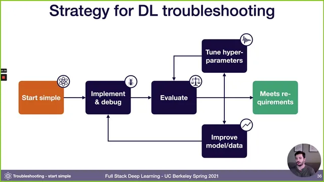
To make debugging less like random stirring and more like controlled diagnosis, the lecture pushes a single mindset: pessimism. Instead of assuming the first attempt is close to correct, it recommends a staged strategy that starts with the simplest possible setup and increases complexity gradually. The workflow is: pick the simplest model and dataset, implement it, get it to run, then overfit a single batch until the loss can be driven arbitrarily close to zero. If that fails, the problem is almost certainly in the implementation or data pipeline (common culprits include corrupted data/labels, silent broadcasting or shape issues, incorrect preprocessing, or over-regularization). Once a single batch can be memorized, compare results against a known reference—ideally an official implementation on a similar dataset, otherwise a benchmark like MNIST, or even simple baselines such as predicting the mean.

After the model is “bug-free enough,” the lecture shifts to deciding what to improve next using bias-variance decomposition. Training error, validation error, and test error are treated as signals: gaps indicate avoidable bias (underfitting), variance (overfitting to training), and validation/test overfitting. When train and test come from different distributions, it recommends using two validation sets—one sampled from the training distribution and one from the test distribution—to quantify distribution shift as an additional error term.

With those diagnostics, improvement priorities follow a sequence: reduce underfitting first (often by increasing model capacity, adjusting regularization, tuning hyperparameters, or adding features), then address overfitting (typically by adding data, using normalization/augmentation, and tuning), then tackle distribution shift via error analysis and targeted data collection or synthetic data, and finally rebalance validation strategy if hyperparameter search has overfit to the validation set. For hyperparameter tuning itself, the lecture recommends starting with sensible defaults (e.g., Adam, a “magic” learning rate, and leaving regularization/normalization out initially to avoid extra bugs), then tuning learning rate first and using course-defined random search to efficiently explore the space before considering Bayesian optimization as projects mature.

Overall, the central message is operational: build in layers, verify each layer with strict sanity checks, and let measured error patterns dictate the next engineering move rather than guessing.