Linear Algebra 11 | Matrices
Based on The Bright Side of Mathematics's video on YouTube. If you like this content, support the original creators by watching, liking and subscribing to their content.
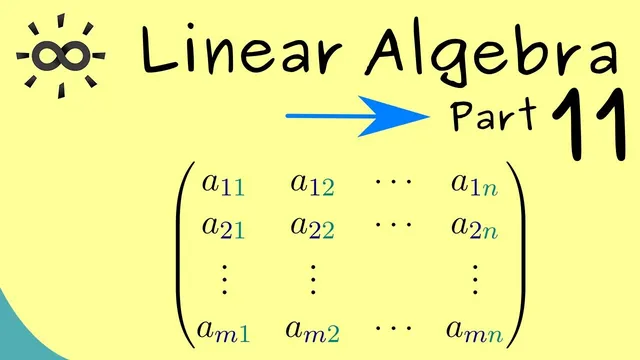
A matrix is a rectangular m-by-n table of numbers, with entries labeled a_{ij} by row i and column j.
Briefing
Matrices enter linear algebra as the tool for solving systems of linear equations—problems that can involve many equations at once. A matrix is fundamentally a rectangular array (a two-dimensional table) of numbers. Its layout is determined by two natural numbers: m rows and n columns. That means the matrix contains m × n entries, typically written as a_{ij}, where i identifies the row and j identifies the column. The bottom-right entry is a_{mn}, and the table need not be square; it can be any m-by-n rectangle.
With that structure in place, the set of all m-by-n matrices with real entries is denoted by R^{m×n}. The “m×n” part signals the fixed shape of the rectangle, while the entries come from the real numbers. The transcript then builds the basic operations needed to treat matrices like vectors: addition and scalar multiplication. Addition is only defined when the two matrices have the same shape. For matrices A and B of size m-by-n, their sum C = A + B is formed entry-by-entry: each entry c_{ij} equals a_{ij} + b_{ij}. A quick example with 2-by-2 matrices shows how the rule works in practice, producing another 2-by-2 matrix.
Scalar multiplication takes a matrix A and a real number λ and produces a new matrix λA of the same shape. Again, the operation is entry-wise: each entry becomes λ·a_{ij}. The key point is that both operations preserve the matrix’s dimensions—so the result stays within the same space R^{m×n}.
These definitions are not just formalities; they make matrices behave like a vector space. Under addition, matrices form an abelian group: addition is associative and commutative, there is a zero matrix (the additive identity) with all entries equal to 0, and every matrix has an additive inverse obtained by negating each entry. Scalar multiplication is compatible with multiplication of scalars, and distributive laws connect scalar multiplication with matrix addition. Because these standard vector-space properties carry over entry-by-entry from real-number arithmetic, matrices can be manipulated using the same kinds of algebraic rules used for vectors.
The practical motivation is saved for later: once matrices can be added and scaled reliably, they become the language for systems of linear equations. The next step is to use matrices to organize those equations and compute solutions efficiently—turning a multi-equation problem into a structured algebraic one.
Cornell Notes
Matrices are rectangular arrays of real numbers organized into m rows and n columns, with entries labeled a_{ij}. The collection of all m-by-n real matrices is written R^{m×n}. Addition and scalar multiplication are defined entry-by-entry: (A+B)_{ij}=a_{ij}+b_{ij} and (λA)_{ij}=λ·a_{ij}, and both operations require the matrices to have the same shape (for addition) while preserving that shape. These operations satisfy the vector-space rules: matrices form an abelian group under addition (including a zero matrix and additive inverses), scalar multiplication is compatible with scalar multiplication, and distributive laws hold. This vector-space structure sets up matrices as the framework for solving systems of linear equations.
How is the size of a matrix determined, and what do the indices mean?
What exactly is the definition of matrix addition, and when is it allowed?
How does scalar multiplication work for matrices?
Why do matrices form a vector space under these operations?
What is the motivation for introducing matrices after defining their operations?
Review Questions
- What conditions must two matrices satisfy for addition to be defined, and how is each resulting entry computed?
- Describe how the additive identity and additive inverse are represented for matrices.
- Explain why entry-wise definitions of addition and scalar multiplication lead to vector-space properties for R^{m×n}.
Key Points
- 1
A matrix is a rectangular m-by-n table of numbers, with entries labeled a_{ij} by row i and column j.
- 2
The set of all m-by-n real matrices is denoted R^{m×n}, where the shape is fixed by m and n.
- 3
Matrix addition is defined only for matrices of the same shape and is computed entry-by-entry: (A+B)_{ij}=a_{ij}+b_{ij}.
- 4
Scalar multiplication multiplies every entry by the same real number: (λA)_{ij}=λ·a_{ij}, preserving the matrix’s dimensions.
- 5
Under addition, matrices form an abelian group, including a zero matrix as the additive identity and a negated-entry matrix as the additive inverse.
- 6
With scalar multiplication and distributive laws, R^{m×n} satisfies vector-space axioms, enabling vector-space style algebra with matrices.
- 7
Matrices are introduced as the framework for solving systems of linear equations in later material.