Linear Algebra 20 | Linear maps induce matrices

TL;DR

Any linear map f: R^n → R^m can be represented as f(x) = A x for a unique m×n matrix A.

Briefing Cornell Notes

Briefing

Every linear map between finite-dimensional real vector spaces can be turned into a unique matrix—so the abstract action of a function becomes a concrete table of numbers, and matrix multiplication can do the work. For a linear map f: R^n → R^m, there exists exactly one m×n matrix A such that for every vector x in R^n, the equality f(x) = A x holds. This matters because it bridges two viewpoints: “linear map” as an operation on vectors, and “matrix” as a computational object.

The key mechanism is how any vector x in R^n decomposes using canonical unit vectors. Writing x as the column vector (x1, …, xn)^T, one can express x as a linear combination of the unit vectors e1, e2, …, en: x = x1 e1 + x2 e2 + … + xn en. Linearity then forces f(x) to split the same way: f(x) = x1 f(e1) + x2 f(e2) + … + xn f(en). That observation immediately implies that knowing the images of the unit vectors is enough to determine f completely. In other words, the entire linear map is encoded by the list of vectors f(e1), f(e2), …, f(en).

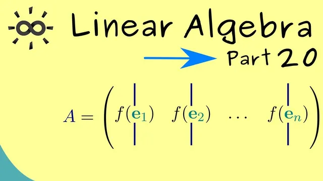
From there, the matrix representation becomes almost inevitable. The m×n matrix A is constructed so that its columns are exactly those images: the first column is f(e1), the second column is f(e2), and so on until the nth column is f(en). With this setup, multiplying A by x reproduces the same linear combination that defines f(x). The existence part of the proof checks this directly: matrix-vector multiplication forms a sum of x_i times the i-th column of A, which—by construction—matches the linearity expansion of f(x).

Uniqueness follows from a contradiction-style argument. Suppose two matrices A and B both represent the same linear map f, meaning f(x) = A x and f(x) = B x for all x. Then A x = B x for every x, so (A − B) x = 0 for all x in R^n. Choosing x to be each unit vector e_i forces every column of (A − B) to be the zero vector, so A − B must be the zero matrix. Therefore A = B, proving there is exactly one matrix representation.

The takeaway is bidirectional: matrices induce linear maps, and linear maps can be translated back into matrices. That equivalence sets up the next step—using matrices to compute and reason about linear transformations efficiently.

Cornell Notes

A linear map f: R^n → R^m is completely determined by what it does to the canonical unit vectors e1, …, en. Because any vector x can be written as x = Σ x_i e_i, linearity gives f(x) = Σ x_i f(e_i). This leads to a unique m×n matrix A whose columns are f(e1), …, f(en), so that f(x) = A x for every x. Existence comes from matching the linear combination produced by matrix-vector multiplication to the linearity expansion of f(x). Uniqueness comes from showing that if two matrices agree on all x, then their difference annihilates every e_i, forcing the matrices to be identical.

Why do the images of the unit vectors f(e1), …, f(en) determine the entire linear map f?

Any x in R^n can be written as x = x1 e1 + x2 e2 + … + xn en. Linearity then forces f(x) = x1 f(e1) + x2 f(e2) + … + xn f(en). So once f(ei) is known for each i, the value of f(x) for every x is fixed.

How is the matrix A constructed from a linear map f: R^n → R^m?

A is an m×n matrix whose columns are the vectors f(e1), f(e2), …, f(en). Concretely, the first column of A equals f(e1), the second equals f(e2), and the last equals f(en). This construction ensures that A x reproduces the same linear combination as f(x).

What does the existence proof rely on when showing f(x) = A x?

Matrix-vector multiplication forms a linear combination of the columns of A with coefficients x1, …, xn. Since the columns of A were defined to be f(e1), …, f(en), the product A x becomes x1 f(e1) + … + xn f(en), which matches f(x) by linearity.

How does the uniqueness argument force two representing matrices to be equal?

If both A and B satisfy f(x) = A x = B x for all x, then (A − B) x = 0 for all x. Taking x = e_i makes (A − B) e_i = 0, which means the i-th column of (A − B) is the zero vector. Since this holds for every i, all columns are zero, so A − B is the zero matrix and A = B.

What is the practical computational benefit of the matrix representation?

Instead of computing f directly from its abstract definition, one can compute f(x) via matrix multiplication A x. This turns linear transformation problems into standard algebra with numbers and operations on vectors.

Review Questions

Given a linear map f: R^n → R^m, how would you compute f(x) using only the values f(e1), …, f(en)?
Why does (A − B) x = 0 for all x imply A = B, and what role do the unit vectors e_i play?
How does the column construction of A (columns equal to f(e_i)) guarantee that A x matches the linearity expansion of f(x)?

Key Points

1
Any linear map f: R^n → R^m can be represented as f(x) = A x for a unique m×n matrix A.
2
Every vector x in R^n decomposes as x = Σ_{i=1}^n x_i e_i using canonical unit vectors.
3
Linearity forces f(x) to split as f(x) = Σ_{i=1}^n x_i f(e_i), so f is determined by f(e_i).
4
The representing matrix A is built by placing f(e1), …, f(en) as its columns.
5
Existence is verified by matching matrix-vector multiplication’s linear combination of columns to the linearity expansion of f(x).
6
Uniqueness follows because if A x = B x for all x, then (A − B) e_i = 0 for each i, making A − B the zero matrix.
7
Matrices and linear maps are interchangeable in finite-dimensional real spaces: each induces the other.

Highlights

A linear map’s entire behavior is encoded in the list of vectors f(e1), …, f(en).

The representing matrix A is formed by using those vectors as columns, making f(x) computable as A x.

Uniqueness comes from testing equality on all vectors—especially the unit vectors—which pins down every column of the matrix.

The proof hinges on the same linear-combination structure appearing in both linearity and matrix-vector multiplication.