Linear Algebra 35 | Rank-Nullity Theorem
Based on The Bright Side of Mathematics's video on YouTube. If you like this content, support the original creators by watching, liking and subscribing to their content.
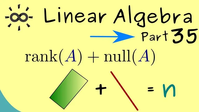
Rank(A) is the dimension of the range (image) of A, and nullity(A) is the dimension of the kernel of A.
Briefing
Rank–nullity theorem is the organizing rule behind how linear maps “trade” dimensions: for any linear map represented by a matrix with n columns, the dimension of its image (rank) plus the dimension of its kernel (nullity) always equals n. In practical terms, when a map collapses some directions in the input space, those lost dimensions reappear as independent directions that get sent to the zero vector. That conservation law matters because it lets students compute unknown ranks or nullities without brute-force counting, and it becomes a key tool for understanding solvability of linear systems.
The discussion begins by defining rank and nullity in geometric terms. For a matrix A, the range (image) is the set of all outputs A x, forming a subspace whose dimension is the rank. Since A maps from R^n to R^m, the rank can’t exceed the number of input directions n or the output ambient dimension m, so rank(A) lies between 0 and min(n, m). Full rank means the rank hits that upper bound. Nullity is defined as the dimension of the kernel: the subspace of vectors x such that A x = 0. Nullity is also a non-negative integer, bounded between 0 and n.
Examples make the bookkeeping concrete. A 1×? matrix with a single row has rank 1 because its columns can span only a one-dimensional subspace. A 2×3 matrix can have rank 2 if its first two columns are linearly independent; then the third column is redundant for spanning the image. In that same 2×3 setup, the rank–nullity relationship appears directly: the map sends R^3 into R^2, so one input dimension is “lost.” The lost direction is identified by a specific vector—adding the three columns yields the zero vector when applied to (1,1,1)—showing that (1,1,1) lies in the kernel. With kernel dimension 1 and rank 2, the sum 1 + 2 matches the original input dimension 3.
The theorem is then stated in general form: for a matrix A with n columns, rank(A) + nullity(A) = n. The proof uses a dimension argument built from bases. Let k be the nullity, so the kernel has a basis {b1,…,bk}. A basis-extension result (the Steinitz exchange lemma) allows those k vectors to be extended to a full basis of R^n by adding n−k vectors {c1,…,c_{n−k}}. The proof then examines the images A c_i to control the dimension of the range. Because the b_i lie in the kernel, their images vanish, so the range is spanned by A c_i, giving an inequality that dim(range(A)) ≤ n−k. The remaining step shows these images are linearly independent: any linear combination of A c_i that lands at zero corresponds to a vector in the kernel, and expressing that vector in the kernel basis forces all coefficients to be zero by linear independence of the full basis. That establishes dim(range(A)) = n−k, i.e., rank(A) = n−k, completing rank(A)+nullity(A)=n.
The takeaway is operational: rank–nullity turns dimension counting into a reliable identity, setting up later work on solving linear equations where kernel structure determines degrees of freedom and rank controls constraints.
Cornell Notes
Rank–nullity theorem links two subspaces tied to a matrix A: the image (range) and the kernel. Rank(A) is the dimension of the range, while nullity(A) is the dimension of the kernel. For a matrix with n columns, the theorem guarantees rank(A) + nullity(A) = n, meaning any loss of dimension in the output must show up as independent directions that map to zero. The proof builds a basis for the kernel, extends it to a basis of R^n, and then shows the images of the added basis vectors form a linearly independent spanning set for the range. This identity is a core tool for analyzing linear systems and understanding how many solutions (or degrees of freedom) to expect.
How are rank and nullity defined for a matrix A, and what bounds do they satisfy?
What does “full rank” mean in this setting?
In the 2×3 example, how does the kernel dimension get identified?
Why does the proof extend a basis of the kernel to a basis of R^n?
How does the proof show dim(range(A)) ≤ n−k and then equality?
What is the practical meaning of rank–nullity when mapping R^3 into R^2?
Review Questions
- If rank(A)=3 for a matrix A with n columns, what must nullity(A) be?
- Explain why vectors in a basis of the kernel contribute nothing to the span of the range after applying A.
- In the proof, what role does linear independence of the extended basis play in proving rank(A)+nullity(A)=n?
Key Points
- 1
Rank(A) is the dimension of the range (image) of A, and nullity(A) is the dimension of the kernel of A.
- 2
For a matrix A with n columns, rank(A) + nullity(A) = n always holds.
- 3
Rank(A) is bounded by 0 ≤ rank(A) ≤ min(n,m) when A maps R^n to R^m.
- 4
Full rank means rank(A)=min(n,m), so the columns span the largest possible subspace.
- 5
Nullity(A) counts independent input directions that collapse to the zero vector under A.
- 6
The proof constructs a basis for ker(A) and extends it to a basis of R^n, then uses images of the added basis vectors to determine dim(range(A)).
- 7
Linear independence of the images A c_i is obtained by translating a zero image back into the kernel and invoking independence of the full basis.