Linear Algebra 37 | Row Operations

Row operations are the reversible matrix moves that make Gaussian elimination possible without losing any information about solutions. Starting from a linear system written as A x = B, the system’s full information sits inside the augmented matrix [A|B]. Any row manipulation can be represented as multiplying by an invertible square matrix M on the left, turning A into a new matrix à = M A and B into Ã_B = M B. Because M is invertible, the transformation can be undone, meaning no solution information is lost—only the form becomes easier to read.

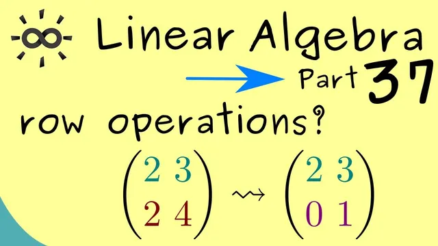
The practical goal is to simplify A into a structure with zeros below the diagonal, creating the “triangle” pattern that makes solving for x straightforward. In the general setting, this simplification is achieved by combining three elementary row operations, each with a clean matrix representation.

First is adding a multiple of one row to another. For an M×N matrix A with rows labeled α_1^T, α_2^T, …, α_M^T, adding row i into row j with a scalar Λ can be encoded using a special matrix Z. Conceptually, Z is built from the identity matrix but with Λ placed in the (j,i) position (with i ≠ j). Multiplying Z A performs the row update: it replaces row j by row j + Λ·row i while leaving other rows unchanged. This Z is invertible because the operation can be reversed by subtracting Λ·row i from row j.

Second is exchanging two rows. Swapping rows i and j is represented by a permutation matrix P_{ij}. Like Z, P_{ij} is constructed from the identity matrix, but with the rows (and corresponding columns) rearranged so that α_i^T and α_j^T trade places. Permutation matrices are invertible, since the swap can be undone by swapping the same two rows again.

Third is scaling a row. Multiplying row i by a nonzero scalar D_i is represented by a diagonal matrix D whose diagonal entries are D_1, …, D_M. Invertibility requires every diagonal entry be non-vanishing; otherwise the transformation would collapse information and could not be reversed.

All row operations—whether row additions, swaps, or scalings—can be combined into a finite product of these invertible matrices. The key invariant is the kernel: for any matrix A, the kernel of M A equals the kernel of A whenever M is invertible. That means row operations do not change which vectors x satisfy A x = 0, and by extension they preserve the solution set structure for systems. The range may change, but the solution-relevant part (the null space) stays fixed. This kernel invariance is the foundational fact that Gaussian elimination relies on in later steps.