Linear Algebra 40 | Row Echelon Form

TL;DR

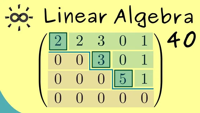
Row echelon form generalizes upper-triangular structure to rectangular matrices using a pivot staircase pattern.

Briefing Cornell Notes

Briefing

Row echelon form turns a messy matrix into a structured one where the “action” happens only at a few key entries called pivots—making it possible to systematically solve linear systems, even when the matrix isn’t square. The defining feature is a row-by-row staircase pattern: any all-zero rows must sit at the bottom, and in each nonzero row the first nonzero entry must appear strictly to the right of the first nonzero entry in the row above. This generalizes the familiar upper-triangular form from square matrices to rectangular ones, and it works because Gaussian elimination naturally produces this pivot staircase.

In the course’s running example, a 4×5 matrix ends up with exactly three pivots. Those pivot positions are the same numbers needed throughout Gaussian elimination, so they determine which variables are “leading” and which are “free.” Once the augmented matrix is in row echelon form, the system’s unknowns split into two categories: variables whose columns contain pivots become leading variables, while variables whose columns have no pivots become free variables. The free variables can take arbitrary real values, and the leading variables are then rewritten as functions of those free choices.

The practical workflow is straightforward. Start with a system Ax = B, convert it to an augmented matrix, and apply Gaussian elimination until the matrix reaches row echelon form. Then identify the pivot columns and non-pivot columns. Move the free variables to the right-hand side (equivalently, treat them as parameters), and use backward substitution to compute the leading variables. If a row in the echelon form ends up as 0 = nonzero (a nonzero entry in the augmented part where the left side is all zeros), the system has no solutions; if it becomes 0 = 0, solutions exist and the free variables generate them.

A concrete example illustrates the method with explicit numbers. After placing the augmented matrix into row echelon form, the system has two free variables, X2 and X5, meaning there are no pivots in their columns. The remaining variables—X1, X3, and X4—are solved in terms of X2 and X5 using backward substitution. The resulting expressions are: - X4 = 2 − 2X5 - X3 = 2 − 3X5 - X1 = 1 − 2X2 + 2X5 With X2 and X5 free to be any real numbers, the solution set contains infinitely many vectors in R^5.

Finally, the solution set can be rewritten as a linear combination: a constant vector plus a part scaled by X2 and another part scaled by X5. That representation makes the geometry clear—here it forms a shifted two-dimensional subspace (a plane-like set) inside the ambient space. The key takeaway is that row echelon form doesn’t just simplify computation; it reveals the degrees of freedom in the system and therefore the structure of the entire solution set.

Cornell Notes

Row echelon form is a matrix layout designed for solving linear systems. It requires that any all-zero rows appear at the bottom and that, moving downward, the first nonzero entry in each row (the pivot) lies strictly to the right of the pivot in the row above. Gaussian elimination produces this form, and the pivot columns determine which variables are leading versus free. Free variables can be chosen arbitrarily; leading variables are then computed as functions of those free choices using backward substitution. In the worked example, X2 and X5 are free, while X1, X3, and X4 are expressed in terms of them, yielding infinitely many solutions that form a shifted two-dimensional subspace.

What exact conditions define a matrix in row echelon form, and why do they matter for solving systems?

A matrix is in row echelon form if (1) any row that is entirely zeros must be located at the bottom, and (2) for each nonzero row, the first nonzero entry (the pivot) must be strictly to the right of the first nonzero entry in the row above. These rules create a staircase structure so pivots can be identified unambiguously row by row, which in turn determines which columns correspond to leading variables and which correspond to free variables.

How do pivot positions translate into “leading” versus “free” variables?

In an augmented matrix, each column corresponds to a variable. If a column contains a pivot, that variable is leading; if a column has no pivot, that variable is free. In the example, there are no pivots in the columns for X2 and X5, so X2 and X5 are free variables. The other variables (X1, X3, X4) are leading and must be solved in terms of the free ones.

What is the step-by-step procedure for turning row echelon form into a full solution set?

First, write the system Ax = B as an augmented matrix. Next, apply Gaussian elimination until the augmented matrix reaches row echelon form. Then identify free variables (non-pivot columns) and leading variables (pivot columns). Move the free variables to the right-hand side (treat them as parameters) and use backward substitution from the bottom row upward to compute leading variables. If a bottom row becomes 0 = nonzero, the solution set is empty; if it becomes 0 = 0, solutions exist.

In the worked numerical example, how are the leading variables expressed in terms of the free variables?

After row echelon form is reached, X2 and X5 are free. Backward substitution yields: X4 = 2 − 2X5, X3 = 2 − 3X5, and X1 = 1 − 2X2 + 2X5. Because X2 and X5 can be any real numbers, each choice produces a different solution vector.

Why does the solution set become a shifted subspace, and what does “two-dimensional” mean here?

Once leading variables are written as linear expressions in the free variables, the full solution vector can be expressed as a linear combination: a constant vector plus terms multiplied by X2 and X5. That structure means the solutions form a shifted subspace. Since there are two free variables (X2 and X5), the solution set has dimension 2, corresponding to a two-parameter family of solutions (infinitely many vectors).

Review Questions

What two structural rules must a matrix satisfy to be in row echelon form, and how do they ensure pivots can be read consistently?
How do you determine which variables are free once the augmented matrix is in row echelon form?
Given pivot and non-pivot columns, how does backward substitution produce expressions for leading variables in terms of free variables?

Key Points

1
Row echelon form generalizes upper-triangular structure to rectangular matrices using a pivot staircase pattern.
2
All-zero rows must be placed at the bottom, and each pivot must appear strictly to the right of the pivot above it.
3
Pivot columns identify leading variables; non-pivot columns identify free variables that can be chosen arbitrarily.
4
Solving Ax = B becomes systematic: convert to an augmented matrix, apply Gaussian elimination to reach row echelon form, then use backward substitution.
5
If a row reduces to 0 = nonzero, the system has no solutions; if it reduces to 0 = 0, solutions exist.
6
Once leading variables are written in terms of free variables, the entire solution set can be expressed as a linear combination of vectors.
7
With k free variables, the solution set forms a shifted k-dimensional subspace and therefore contains infinitely many solutions when k > 0.

Highlights

Row echelon form is defined by a strict “first nonzero entry moves right” rule plus the requirement that zero rows sink to the bottom.

Pivot positions simultaneously encode the Gaussian elimination structure and the variable classification into leading versus free.

Backward substitution after row echelon form turns a system into explicit formulas for leading variables as functions of free variables.

In the example, X2 and X5 are free, producing infinitely many solutions and a shifted two-dimensional solution set.

Topics

Row Echelon Form
Gaussian Elimination
Pivot Variables
Free Variables
Backward Substitution