Linear Regression with TensorFlow.js
Based on Venelin Valkov's video on YouTube. If you like this content, support the original creators by watching, liking and subscribing to their content.
Simple linear regression models house price as **price ≈ B·X + a**, learning **B** (slope) and **a** (intercept) from training data.
Briefing
Linear regression in TensorFlow.js is built to learn the parameters of a straight-line (or hyperplane) relationship between house features and price—then it’s judged by how closely its predictions match real values. In the simple case, the model assumes price follows a line: **price ≈ B·X + a**, where **B** acts like a slope controlling how strongly living area (X) changes price, and **a** shifts where the line crosses the y-axis. The training goal is to automatically find **B** and **a** that best fit the preprocessed dataset, so the model can predict prices for new houses (for example, around **$200k** for **2,000 square feet** in the example).
When more than one feature is available, the approach expands into **multiple linear regression** by replacing the single slope with a set of **weights (W)**—one per feature—so the model can combine several inputs at once. The core training loop stays the same: predictions are compared against true prices using a loss/metric, and the model parameters are adjusted to reduce error. The transcript emphasizes **root mean squared error (RMSE)** as the primary diagnostic measure, since it penalizes larger mistakes more heavily by squaring the differences between predicted and actual prices and then taking the square root. Because TensorFlow.js doesn’t provide RMSE directly in the setup shown, RMSE is computed from **mean squared error** during training.
Implementation starts with a function (named **trainLinearModel**) that builds a TensorFlow.js **sequential** model. For simple linear regression, the model uses an input shape derived from the training tensor and a single output unit, meaning it learns one parameter for the relationship. The model is compiled with **SGD (stochastic gradient descent)** using a learning rate of **0.001**, and it tracks **mean squared error** (converted to RMSE) plus **mean absolute error** (MAE) to show how far predictions deviate from real prices in dollar terms.
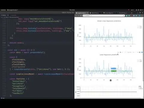
Training uses **fit()** with a batch size of **32**, **100 epochs**, and a validation split of **10%**. A callback runs at the end of each epoch to record training and validation RMSE and MAE, which are then plotted into two HTML containers (one for error over epochs and one for MAE).
A second run trains a more complex version: multiple linear regression with **units equal to the number of features**, but the transcript notes a shape issue—an additional layer is added to ensure the model outputs a single predicted price value. An activation function is also introduced to restore the expected error tracking behavior.
After both models train, predictions are generated on a test set and compared visually. The results show that the **simple linear regression and the multiple linear regression predictions are nearly identical** in this case, including similar outputs such as predicting roughly **$180k** for a sample house. The takeaway is practical: adding complexity (more parameters/features) does not automatically improve performance; preparation and training quality can matter as much as model size.
Cornell Notes
The transcript builds linear regression in TensorFlow.js to predict house prices from preprocessed features. Simple linear regression learns two parameters—slope **B** and intercept **a**—to fit a straight-line relationship between living area and price. Multiple linear regression generalizes this by learning a set of weights **W** for multiple features, but it still aims to minimize prediction error. Training uses **SGD** with learning rate **0.001**, tracks **RMSE** (computed from mean squared error) and **MAE**, and evaluates on a validation split and a test set. In the final comparison, the simple and multiple models produce nearly identical predictions, suggesting that more complexity doesn’t guarantee better results if data prep or training isn’t improved.
How does simple linear regression translate into a TensorFlow.js model structure?
Why compute RMSE manually instead of using a built-in metric?
What training configuration is used, and how are metrics recorded over time?
What changes when moving from simple to multiple linear regression?
What does the final prediction comparison reveal about model complexity?
Review Questions
- In the transcript’s setup, how is RMSE derived from mean squared error, and why is that useful for regression diagnostics?
- What specific architectural adjustment is made to ensure the multiple-feature model outputs a single predicted price?
- Why might a multiple linear regression model perform no better than a simple linear regression model in the final test comparison?
Key Points
- 1
Simple linear regression models house price as **price ≈ B·X + a**, learning **B** (slope) and **a** (intercept) from training data.
- 2
Multiple linear regression replaces the single slope with feature-specific **weights (W)**, but still aims to minimize prediction error.
- 3
Training uses **SGD** with learning rate **0.001**, and tracks both **RMSE** (computed from MSE) and **MAE**.
- 4
RMSE is computed manually because RMSE isn’t provided directly in the metric setup used; RMSE is **sqrt(MSE)**.
- 5
Training runs with **batch size 32**, **100 epochs**, and **10% validation split**, while callbacks log metrics each epoch.
- 6
A shape/output mismatch can occur when increasing units for multiple features; adding a final layer that outputs **one unit** fixes prediction shape.
- 7
More model complexity doesn’t guarantee better accuracy: the simple and multiple models end up producing nearly identical predictions in the test comparison.