Manifolds 17 | Examples of Smooth Maps
Based on The Bright Side of Mathematics's video on YouTube. If you like this content, support the original creators by watching, liking and subscribing to their content.
Smoothness of a manifold map is checked locally by composing with charts to obtain a Euclidean coordinate map and verifying differentiability (C∞).
Briefing
Smooth maps between manifolds can be checked chart-by-chart by translating the problem into ordinary maps between Euclidean spaces. Using that method, two canonical constructions—embedding a sphere into Euclidean space and projecting a sphere onto real projective space—turn out to be infinitely differentiable (C∞).
The first example starts with the 2-sphere S2 viewed as a subset of R3. The inclusion map I sends each point x in S2 to the same point in R3. Topologically, this is continuous by construction. To test smoothness, the discussion uses charts: on S2, the southern-hemisphere chart H3− identifies points with coordinates (x1, x2) in R2, while the inverse chart reconstructs the missing third coordinate using a square root. In the target R3, the relevant local description is essentially the identity. Composing the charts with the inclusion map yields a local Euclidean map that takes (x1, x2) to (x1, x2, …) with the third component recovered smoothly. Because the resulting coordinate expression is differentiable and can be shown to be C∞, the inclusion map I is a smooth map of manifolds. The same reasoning applies on other hemispherical charts, so smoothness holds globally.
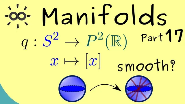
The second example replaces S2 with real projective space P2, defined as a quotient of S2 by identifying antipodal points: x ~ y exactly when y equals x or −x. The canonical projection q sends each point of S2 to its equivalence class in P2 and is continuous by the definition of the quotient topology. Smoothness again requires local chart computations. The approach uses the same southern-hemisphere chart H3− on S2, and a corresponding chart K on P2 (from earlier material) that uses coordinates formed by ratios like x1/x3 and x2/x3. These ratios are only defined where x3 ≠ 0, which matches the chart’s domain.
Locally, the smoothness question reduces to whether the composed map from R2 to R2—K ∘ q ∘ (H3−)^{-1}—is differentiable. Tracing the composition shows that (H3−)^{-1} reconstructs a point on the sphere with a square-root expression for x3, q then passes to the equivalence class without changing the local coordinates, and K converts the class back into R2 using division by that nonzero x3 value. The coordinate formulas therefore involve dividing by a square root, but since the denominator stays nonzero on the chart domain, partial derivatives exist and the map is C∞. Covering the sphere with corresponding charts extends the conclusion across all points.
Together, these two constructions provide concrete, chart-based examples of smooth maps: the canonical embedding of S2 into R3 and the canonical quotient projection from S2 onto P2 are both smooth and infinitely differentiable.
Cornell Notes
Smoothness between manifolds is verified by converting the map into a local Euclidean map using charts. For the inclusion I: S2 → R3, the southern-hemisphere chart H3− on S2 and the identity description in R3 produce a coordinate expression where the missing coordinate is recovered via a square root; this yields a C∞ local map, and the same works on other hemispheres. For the quotient projection q: S2 → P2, antipodal points are identified (x ~ ±x). Using H3− on S2 and a projective chart K with coordinates like x1/x3 and x2/x3 (valid when x3 ≠ 0), the composition K ∘ q ∘ (H3−)^{-1} becomes a differentiable R2 → R2 map involving division by a nonzero square-root term, giving C∞ smoothness. These two canonical maps are therefore smooth everywhere on their manifolds.
How does one check whether the inclusion map I: S2 → R3 is smooth?
Why is the inclusion map automatically continuous, and why isn’t that enough for smoothness?
What defines real projective space P2 in this discussion, and what is the canonical projection q?
How does the projective chart K on P2 relate to the ratios x1/x3 and x2/x3?
Why does the composition K ∘ q ∘ (H3−)^{-1} become C∞ on its chart domain?
Review Questions
- In the inclusion map example, which coordinate is reconstructed using a square root, and why does that matter for smoothness?
- For the quotient projection q: S2 → P2, what role does the condition x3 ≠ 0 play in the projective chart K?
- How does the chart-by-chart method turn a manifold smoothness question into an ordinary differentiability question between maps R2 → R2?
Key Points
- 1
Smoothness of a manifold map is checked locally by composing with charts to obtain a Euclidean coordinate map and verifying differentiability (C∞).
- 2
The inclusion map I: S2 → R3 is smooth because the local coordinate expression recovers the missing coordinate via a square-root formula and remains C∞ on each chart domain.
- 3
Real projective space P2 is formed by identifying antipodal points on S2 using the equivalence relation x ~ ±x.
- 4
The canonical projection q: S2 → P2 is continuous by quotient topology, but smoothness still requires chart-level verification.
- 5
A projective chart K uses coordinates like x1/x3 and x2/x3, so it is defined only where x3 ≠ 0.
- 6
On the chart domain where x3 stays nonzero, the composed map K ∘ q ∘ (H3−)^{-1} is C∞, and covering with charts extends smoothness across the manifold.