Manifolds 24 | Differential in Local Charts

TL;DR

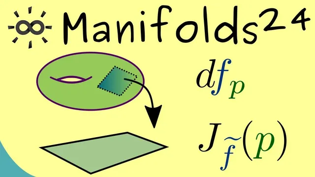
A smooth manifold map F: M → N can be studied locally by converting it into an ordinary map between Euclidean spaces using charts.

Briefing Cornell Notes

Briefing

Manifolds calculus doesn’t replace ordinary multivariable calculus—it reproduces it once everything is expressed in local coordinates. For a smooth map F: M → N between smooth manifolds, the differential at a point P can be computed in local charts using the same Jacobian machinery familiar from R^n. The key move is to translate the abstract tangent vector at P into a concrete vector in Euclidean space via the chart homeomorphisms, apply the ordinary chain rule, and then translate back.

Concretely, pick charts around P and around F(P). If H is a chart map from an open neighborhood of P in M to an open set in R^n, and K is a chart map from an open neighborhood of F(P) in N to an open set in R^m, then the smoothness of F is equivalent to the smoothness of the coordinate representation F~ = K ∘ F ∘ H^{-1}: R^n → R^m. The differential DF at P is defined using tangent vectors as equivalence classes of curves, so one starts with an abstract tangent vector v ∈ T_P M, represents it by a curve γ through P, and feeds it into DF.

When the tangent vector is pushed through the chart K, it becomes a concrete derivative in R^m. This is where the ordinary chain rule enters: the coordinate map F~ is an ordinary differentiable map between Euclidean spaces, so its differential is represented by the Jacobian matrix J_{F~}(H(P)). The computation yields a product structure: the Jacobian matrix of F~ multiplies the differential of the chart map H (evaluated at the curve parameter value corresponding to P). After that multiplication, the result is converted back into an abstract tangent vector in T_{F(P)}N using the inverse chart correspondence.

The upshot is a clean local formula. In local charts, the differential of the manifold map F is given by “chart inverse” composed with the Jacobian matrix of the coordinate representation and then composed with the differential of the domain chart. In shorthand, this is the familiar pattern: dF = d(K^{-1}) · J_{F~} · dH. That identity explains why the earlier, more abstract definition of the differential using tangent vectors and curves wasn’t arbitrary—it was precisely designed so that, in coordinates, it matches the standard multivariable differential.

This local-chart viewpoint matters because it bridges two worlds: abstract geometry on manifolds and concrete computation with Jacobians. Once the differential is understood this way, the rest of manifold calculus can proceed with the same computational tools, just expressed through charts and their derivatives. The discussion sets up the next step: continuing the differential calculus on manifolds using this coordinate-compatible definition.

Cornell Notes

A smooth map between manifolds can be differentiated using the same Jacobian-based rules as in multivariable calculus, once local charts are used. Given charts H around P in M and K around F(P) in N, the coordinate version F~ = K ∘ F ∘ H^{-1} is an ordinary smooth map from R^n to R^m. The differential DF at P is defined via tangent vectors represented by curves, but in charts those tangent vectors become concrete derivatives. Applying the ordinary chain rule to F~ shows that the differential in local coordinates is represented by a Jacobian matrix multiplied by the derivative of the chart map H, with chart inverses used to translate back to abstract tangent vectors. This confirms that the abstract manifold definition of the differential matches the classical one in local coordinates.

How do local charts turn an abstract manifold map F: M → N into an ordinary multivariable map?

Choose a chart H from a neighborhood of P in M to an open set in R^n, and a chart K from a neighborhood of F(P) in N to an open set in R^m. Then form the coordinate representation F~ = K ∘ F ∘ H^{-1}. Smoothness of F is equivalent to smoothness of F~ as a map between Euclidean spaces R^n → R^m.

Why does the Jacobian matrix appear in the formula for the differential on manifolds?

In charts, the differential of the coordinate map F~ is exactly the ordinary differential of a map R^n → R^m. That ordinary differential is represented by the Jacobian matrix J_{F~} evaluated at the point corresponding to P, namely at H(P) (or equivalently at the curve parameter value giving P). The manifold differential inherits this Jacobian because tangent vectors are translated into concrete Euclidean directions via the charts.

What role does the chain rule play in the manifold differential computation?

The computation follows the same structure as the Euclidean chain rule: the coordinate map is a composition K ∘ F ∘ H^{-1}. When a tangent vector at P is pushed through H, the derivative of H contributes a factor; when the tangent vector is then mapped through F~ to the target coordinates, the Jacobian of F~ contributes the main linear approximation. The resulting linear map is then converted back to an abstract tangent vector using the inverse chart.

How is the abstract tangent vector at P handled concretely in the calculation?

An abstract tangent vector v ∈ T_P M is represented using a curve γ with γ(0) = P. Applying DF to v corresponds to applying DF to the equivalence class determined by γ. Under the chart H, this curve becomes a curve in R^n, so the tangent vector becomes an actual derivative in Euclidean space, allowing the use of standard Jacobian/chain-rule computations.

What is the local-coordinate “shape” of the differential dF?

In local charts, the differential takes the form dF = d(K^{-1}) · J_{F~} · dH. The Jacobian J_{F~} represents the linearization of the coordinate map F~; dH translates tangent vectors from the manifold’s chart coordinates into Euclidean coordinates; d(K^{-1}) translates the result back into the target manifold’s abstract tangent space.

Review Questions

Given charts H and K, write the coordinate map F~ and state what property of F is equivalent to smoothness of F~.
In local coordinates, where is the Jacobian matrix J_{F~} evaluated relative to the point P?
Explain why the abstract definition of the differential using curves must match the Euclidean differential when expressed in charts.

Key Points

1
A smooth manifold map F: M → N can be studied locally by converting it into an ordinary map between Euclidean spaces using charts.
2
With charts H near P and K near F(P), the coordinate representation is F~ = K ∘ F ∘ H^{-1}: R^n → R^m.
3
The manifold differential DF at P is defined using tangent vectors represented by curves through P.
4
In local coordinates, DF is computed using the ordinary chain rule applied to F~.
5
The Jacobian matrix of the coordinate map F~ provides the linear approximation in Euclidean coordinates.
6
The final result is translated back to abstract tangent vectors using the inverse chart maps, yielding a local formula of the form dF = d(K^{-1}) · J_{F~} · dH.

Highlights

The differential on manifolds matches the multivariable differential once everything is expressed in local charts.

The Jacobian matrix enters because the coordinate version F~ is an ordinary map R^n → R^m.

Tangent vectors defined abstractly via curves become concrete derivatives after applying chart maps.

A local formula emerges: dF = d(K^{-1}) · J_{F~} · dH, showing the abstract definitions were built to agree with classical calculus.

Topics

Differential in Local Charts
Manifold Tangent Vectors
Coordinate Representations
Jacobian Matrix
Chain Rule on Manifolds