Manifolds 38 | Integration for Differential Forms

Integration on manifolds becomes natural once differential forms are treated as “density × volume element,” turning the familiar idea of summing mass into a coordinate-free geometric operation. The core move is to reinterpret an ordinary integral as the total mass obtained by slicing a line into tiny intervals, weighting each slice by a density value, and then taking a limit as the slices shrink. In one dimension, this is visualized by rectangles: the integral accumulates f(x)·Δx, and the notation ∫ f(x) dx reflects that Δx becomes dx in the limiting process. The same mass-summing picture extends to higher dimensions by replacing intervals with small regions (rectangles in the plane), so f(x,y)·ΔA becomes the local contribution, and ΔA turns into the appropriate area element.

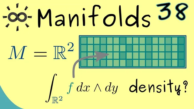
That “density” viewpoint also clarifies why differential forms are the right language for curved spaces. On flat R², a two-dimensional integral can be written using the standard area element dx∧dy. A differential 2-form Ω assigns to each point p on the manifold an alternating 2-form on the tangent space T_pM; in the R² case, Ω can be represented as Ω_p = F(p)·dx∧dy, where F(p) plays the role of the density at p. When two tangent vectors V and W are inserted into Ω, the wedge product dx∧dy produces the determinant of their components, so Ω(V,W) = F(p)·det(V,W). That determinant is exactly the oriented area factor in the tangent plane, meaning Ω already packages “density times area.” With that packaging, the integral can be written succinctly as ∫_M Ω, without separately writing dx dy—because the volume element is built into the form itself.

The key insight for manifolds is that curvature changes what “volume” means locally. Even when the density varies from point to point, the volume element can also vary because it lives in the tangent space at each point. On a curved manifold, the tangent spaces differ from point to point, so the differential form must account for both the density function and the local geometric area/volume measurement supplied by the form. This is why the integral of a differential form generalizes the usual integral: it keeps the same mass-summing intuition, but replaces fixed coordinate volume elements with the tangent-space volume elements encoded by wedge products.

The transcript also situates this within integration theory by contrasting Riemann and Lebesgue integrals. Both ultimately agree on smooth functions, but the Lebesgue approach is more general and better suited to broader classes of functions. Still, the geometric “density” picture is the bridge to manifolds: once integrals are understood as accumulating local contributions weighted by density and measured by the correct volume element, extending from R to R² and then to general manifolds becomes a matter of using differential forms and their tangent-space definitions. The practical construction of the manifold integral via local charts is deferred to the next installment.