Manifolds 47 | Tangent Space and Orientation on the Boundary

A manifold’s boundary needs its own tangent-space and orientation conventions—because Stokes’ theorem links integrals over a manifold to integrals over its boundary, and the sign depends on how “outward” directions are chosen. The core move is to define tangent vectors at boundary points using curves that either approach the boundary point from inside the manifold, leave it, or run along the boundary itself. That distinction produces three kinds of tangent vectors: inward-pointing, outward-pointing, and tangents that lie entirely within the boundary.

For a point Q on the boundary ∂M, the tangent space T_QM is built from equivalence classes of differentiable curves that pass through Q, but the curves are allowed to stop at Q. Concretely, curves that end at Q (denoted C_Q^-), curves that start at Q (denoted C_Q^+), and curves that remain on the boundary all lead to different directional tangent vectors. Using charts, the derivative at the boundary point is computed in local coordinates (involving a half-space model when the chart is adapted to the boundary). The tangent space is then the set of equivalence classes of all such curves, while subsets carve out the geometry: T_QM^+ corresponds to outward-pointing vectors (curves ending at Q), T_QM^- corresponds to inward-pointing vectors (curves starting at Q), and the intersection T_QM^+ ∩ T_QM^- is exactly the tangent space of the boundary manifold itself.

Once a Riemannian metric is in place, the boundary gains a canonical geometric structure. If M is a smooth Riemannian manifold with boundary, the metric restricts to the boundary, making ∂M a Riemannian manifold without boundary. More importantly, ∂M sits inside M as a submanifold, so at each boundary point Q there is a well-defined outward unit normal vector n(Q). This normal vector lies in the orthogonal complement of T_Q(∂M) inside T_QM, has length 1 under the Riemannian metric, and varies continuously with Q. The existence of this outward-pointing unit normal field is what makes the boundary’s orientation unambiguous.

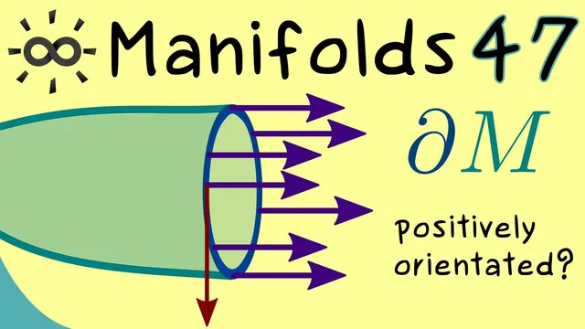
Orientation is then transferred from M to ∂M using a basis rule. Suppose M has an orientation, and at a boundary point Q there is a basis of tangent vectors for T_Q(∂M) (one dimension lower than M). That basis is declared positively oriented relative to M if, after prepending the outward unit normal vector n(Q) to the boundary basis, the resulting ordered basis of T_QM is positively oriented. In the common low-dimensional picture—where M is two-dimensional and ∂M is one-dimensional—this means the boundary’s “positive direction” is the one that pairs with the outward normal to match the manifold’s orientation. Because n(Q) depends continuously on Q, the induced orientation on ∂M is consistent across the boundary. That fixed sign convention is essential for Stokes’ theorem, where integrals over M and over ∂M must match without ambiguity.