Manifolds 48 | Stokes's Theorem as the Fundamental Theorem of Calculus

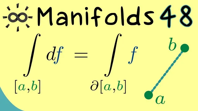
Stokes’s theorem emerges as a “fundamental theorem of calculus” for manifolds once orientation is handled correctly—down to the zero-dimensional boundary points. The key move is rewriting the one-dimensional identity

∫(a→b) df = f(b) − f(a)

as an equality between an integral of a differential form over a manifold and an integral of a related form over its boundary. That rewrite depends entirely on how positive and negative orientations are assigned, including what happens when the boundary is just a pair of points.

The discussion starts by recalling how integration on an orientable manifold M is defined using a chosen positive orientation and a volume form ω. In a chart U, ω becomes an ordinary top-degree form in R^n, and the manifold integral is computed by integrating the corresponding component function over the flattened domain. If a chart reverses orientation—meaning it maps the manifold’s positive orientation to the negative orientation in R^n—then the integral must pick up a minus sign to keep the overall definition independent of chart choice. Flipping the manifold’s orientation globally also flips the sign of the integral.

That sign bookkeeping becomes crucial for manifolds with boundary. The boundary ∂M inherits its orientation from M using the outward-pointing unit normal vector: a basis is positively oriented on the boundary exactly when appending the outward normal yields a positively oriented basis in the tangent space of M. The same logic extends to negatively oriented bases by flipping both sides. The treatment then tackles a subtle edge case: zero-dimensional manifolds. Since the tangent space at a point has an empty basis, “orientation” would otherwise be undefined. The solution is to assign two possible orientations to the empty basis so that boundary inheritance still works. This matters because the boundary of a 1D interval is two points.

With that foundation, the transcript connects the standard fundamental theorem of calculus to Stokes’s theorem in one dimension. Treating the interval [a,b] as a 1D manifold with boundary, its boundary consists of the points a and b with opposite induced orientations: b is positive and a is negative (because the outward normal points in opposite directions at the two ends). For a smooth function f on the interval, the differential df is a 1-form. In the 1D setting, df corresponds to f′(x) dx, so integrating df over the interval gives the usual result f(b) − f(a).

Finally, the same expression is recovered by integrating a 0-form over the boundary. A 0-form is just a smooth function, and integrating it over a zero-dimensional manifold means evaluating the function at the points and summing with orientation signs. Because a carries negative orientation and b carries positive orientation, the boundary integral becomes −f(a) + f(b), matching the integral of df. This is presented as the one-dimensional prototype of Stokes’s theorem: the exterior derivative d “moves” from the integrand to the boundary. The next step, reserved for later videos, is defining an exterior derivative for higher-degree forms and proving the general higher-dimensional Stokes theorem.