Multidimensional Integration 4 | Fubini's Theorem in Action

TL;DR

Fubini’s theorem applies directly when the integration domain is a Cartesian product A×B in R^{n+m}.

Briefing Cornell Notes

Briefing

Fubini’s theorem becomes usable even when the integration region isn’t a rectangle: extend the function by zero outside the curved domain, then apply the theorem to the resulting rectangular setup. That single move—“rectangularize the domain by zero-extension”—turns a hard-looking multidimensional integral into an iterated pair of simpler one-dimensional integrals, with the option to choose the order that makes the zeros easiest to handle.

The discussion starts by recalling the conditions behind Fubini/Tonelli: for a measurable function on a Cartesian product set A×B in R^{n+m}, the (n+m)-dimensional integral can be computed as an iterated integral over A and B, and the order of integration does not matter when the function is either nonnegative or absolutely integrable. The catch is that this direct method requires the domain to be a Cartesian product. When the region is curved—like a subset U of R^2 bounded by a parabola—Fubini’s theorem can’t be applied as-is.

The workaround is to embed the curved region U inside a rectangle A×B and define a new function f_tilda that matches the original function f on U but equals 0 outside U. This extension preserves the integral: integrating f_tilda over the rectangle gives the same value as integrating f over the original region, because the added area contributes nothing. Once the domain is rectangular, Fubini’s theorem applies, and the iterated integrals often simplify dramatically because one of the inner integrals becomes zero whenever the variable falls outside the y-range determined by the boundary of U.

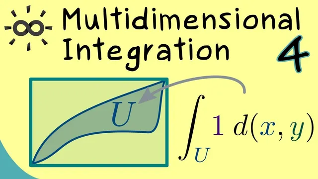
An explicit R^2 example makes the method concrete. The region U is described as the set under the curve y = 3 − x^2, with x running from 0 to 1. Geometrically, taking the integrand to be the constant function f(x,y)=1 means the double integral over U measures the area of U (equivalently, the “volume under the surface” in a 3D visualization).

After extending to a rectangle, the y-limits become dependent on x: for each x in [0,1], y ranges from 1 up to 3 − x^2 (with the integrand effectively zero outside that band). Choosing to integrate with respect to x last is convenient because the inner integral immediately reflects where the function is nonzero. The remaining computation reduces to a single one-dimensional integral: the upper boundary minus the lower boundary, leaving an integral that evaluates to 5/3.

The takeaway is practical: when the region isn’t rectangular, zero-extend the integrand to a rectangle, apply Fubini, and exploit the resulting zeros to collapse the work down to one-dimensional integration. The area of the example region U comes out to 5/3, illustrating how the theorem “works in action” for non-Cartesian domains.

Cornell Notes

Fubini’s theorem computes integrals over rectangular domains A×B as iterated one-dimensional integrals, with integration order not affecting the result under standard conditions (nonnegative or absolutely integrable functions). When the region U is not a Cartesian product, the method still works by extending the integrand: define f_tilda = f on U and f_tilda = 0 outside U within a containing rectangle. This preserves the integral because the added area contributes nothing. After rectangularization, Fubini applies, and the dependence of the boundary on one variable turns the inner integral into a simple “upper minus lower” expression. In the worked example under y = 3 − x^2 for x∈[0,1] with integrand 1, the area of U evaluates to 5/3.

Why can’t Fubini’s theorem be applied directly to a curved region U in R^2?

Fubini’s theorem requires the function’s domain to be a Cartesian product A×B. A curved region like the set under y = 3 − x^2 (with x between 0 and 1) is generally not expressible as A×B, so the theorem’s standard iterated-integral setup doesn’t match the geometry.

How does zero-extension turn a non-rectangular region into a rectangular one?

Pick intervals A and B so that U sits inside A×B. Define f_tilda(x,y)=f(x,y) when (x,y)∈U, and set f_tilda(x,y)=0 for points in A×B but outside U. Because f_tilda contributes zero outside U, the integral of f_tilda over A×B equals the integral of f over U.

What simplification happens inside the iterated integrals after zero-extension?

The inner integral often becomes zero whenever the variable falls outside the y-range (or x-range) determined by the boundary of U. In the example, for each x in [0,1], y only contributes between the lower bound and the upper bound 3 − x^2; outside that band, f_tilda is zero, so the integrand effectively vanishes.

In the example with integrand 1, what does the double integral represent geometrically?

With f(x,y)=1, the double integral over U measures the area of U. The 3D interpretation is “volume under the surface z=1 above the region U in the xy-plane,” which collapses to area because the height is constant.

How does the example lead to the final value 5/3?

After rectangularization, the y-integral becomes (upper boundary − lower boundary) because the integrand is 1 on the allowed band. Using the boundary y up to 3 − x^2 (and the stated lower boundary), the remaining one-dimensional integral over x evaluates to 5/3.

Review Questions

What conditions on f (nonnegative vs integrable/absolute integrability) are needed for Fubini/Tonelli to justify swapping or computing iterated integrals?
Describe the exact definition of f_tilda used to extend an integrand from a curved region U to a rectangle A×B, and explain why the integral is unchanged.
In the worked example, why does the inner integral reduce to an “upper minus lower” expression rather than requiring a more complicated integrand?

Key Points

1
Fubini’s theorem applies directly when the integration domain is a Cartesian product A×B in R^{n+m}.
2
When the region U is not rectangular, embed it in a rectangle A×B and define a zero-extended integrand f_tilda that equals f on U and 0 outside U.
3
Zero-extension preserves the original integral because the added region contributes nothing.
4
After rectangularization, iterated integration can exploit where f_tilda is identically zero, often making one order of integration simpler than the other.
5
Using a constant integrand f=1 turns a double integral over U into the geometric area of U.
6
In the example region under y=3−x^2 with x∈[0,1], the area computed via this method is 5/3.

Highlights

Zero-extension is the key trick: extend the integrand by 0 outside the curved region so the domain becomes rectangular.

Once the domain is rectangular, Fubini’s theorem applies and the dependence of boundaries on one variable collapses the inner integral.

With f(x,y)=1, the double integral over U is literally the area of U.

For the region under y = 3 − x^2 from x=0 to x=1 (with the given lower boundary), the area comes out to 5/3.

Topics

Fubini’s Theorem
Zero-Extension
Iterated Integrals
Area Under a Curve
Non-Rectangular Domains