Multidimensional Integration 6 | Example for Change of Variables

TL;DR

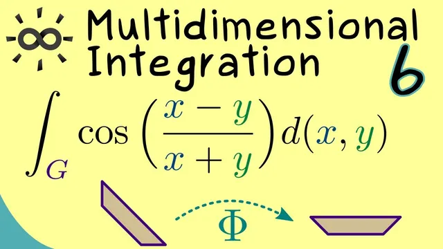
Rewrite the integrand’s fraction (x − y)/(x + y) by selecting u = x − y and v = x + y so the cosine becomes cos(u/v).

Briefing Cornell Notes

Briefing

A two-dimensional change of variables turns a tricky cosine integral over a polygonal region into a pair of one-dimensional integrals that can be finished with a simple antiderivative. The key move is mapping the original coordinates (x, y) to new variables (u, v) using the transformation u = x − y and v = x + y, which straightens the integration region so one variable has clean bounds.

The starting point is a double integral of the form ∫∫_G cos((x − y)/(x + y)) dA, where the domain G in the xy-plane is defined by several inequalities. After rewriting the “outer” inequalities, the region is shown to lie entirely in the first quadrant (x ≥ 0 and y ≥ 0). The remaining constraints reduce to a wedge between two lines: y ≥ 1/2 − x and y ≤ 1 − x. Geometrically, G is a triangular region bounded by those linear relationships.

To apply the change of variables formula, the transformation (x, y) ↦ (u, v) is chosen to match the expression inside the cosine. The Jacobian matrix of (u, v) with respect to (x, y) is computed from u = x − y and v = x + y, giving determinant det(J) = 2 everywhere. That constant determinant means the area-scaling factor in the formula is just |det(J)| = 2, so the integral picks up a simple multiplicative adjustment.

The inequalities defining G are then translated into the uv-plane. From the definitions, u and v relate back to x and y via u + v = 2x and v − u = 2y. Since x and y are nonnegative on G, it follows that u + v ≥ 0 and v − u ≥ 0, which can be rewritten as v ≥ −u and v ≥ u. Meanwhile, the original constraints involving x + y become bounds on v itself: v lies between 1/2 and 1. Putting these together, the image region fi(G) becomes a strip in v with linear boundaries in u, namely u ranges between −v and v.

With the transformed region in hand, the integral splits cleanly using Fubini’s theorem. The outer integral runs over v from 1/2 to 1, and for each fixed v, the inner integral runs over u from −v to v. The inner integral uses an antiderivative of cos(u/v) with respect to u; differentiating sin(u/v) produces a factor 1/v, so multiplying by v cancels it. Evaluating at u = v and u = −v yields a sine difference that collapses using odd/even symmetry: the result simplifies to a constant multiple of sin(1) times an elementary v-integral.

Carrying out the remaining one-dimensional integration over v produces the final value: the original double integral equals 3/8 · sin(1). The example demonstrates how a carefully chosen coordinate transformation can preserve the region’s structure while making the bounds separable, turning a two-variable problem into a straightforward computation.

Cornell Notes

The integral involves cos((x − y)/(x + y)) over a polygonal region G in the first quadrant. By switching to variables u = x − y and v = x + y, the cosine’s argument becomes u/v, and the Jacobian determinant is constant: |det(J)| = 2. Translating the inequalities defining G into uv-coordinates shows that v ranges from 1/2 to 1, while u ranges between −v and v. That separable description lets the double integral be evaluated as an inner integral in u and an outer integral in v. The u-integral uses an antiderivative involving sin(u/v), and symmetry collapses the sine terms, leaving a simple v-polynomial integral. The final result is (3/8)·sin(1).

Why choose u = x − y and v = x + y for this problem?

Because the integrand contains (x − y)/(x + y) inside the cosine. With u = x − y and v = x + y, the argument becomes u/v directly, so the substitution removes the complicated fraction and turns cos((x − y)/(x + y)) into cos(u/v).

How does the Jacobian affect the integral, and why is it easy here?

The change of variables formula multiplies by |det(J)|, where J is the Jacobian of (u, v) with respect to (x, y). Here u = x − y and v = x + y, so the partial derivatives are simple and det(J) = 2 everywhere. A constant determinant means the scaling factor is just 2, not a function of position.

How are the bounds on G converted into bounds on the new region in the uv-plane?

The original constraints include x + y between 1/2 and 1, which becomes v ∈ [1/2, 1]. Also, x ≥ 0 and y ≥ 0 translate using u + v = 2x and v − u = 2y. Those inequalities imply u + v ≥ 0 and v − u ≥ 0, which rearrange to v ≥ u and v ≥ −u. Together, for each fixed v, that means u ∈ [−v, v].

What does Fubini’s theorem buy after the region is transformed?

Once the region is described as u between −v and v, with v between 1/2 and 1, the double integral becomes an iterated integral: ∫_{v=1/2}^{1} ∫_{u=−v}^{v} (cos(u/v) · |det(J)|) du dv. This separability turns the two-variable problem into a manageable inner u-integral followed by a simple outer v-integral.

How does the inner integral of cos(u/v) work out cleanly?

An antiderivative with respect to u is v·sin(u/v), because d/du[sin(u/v)] = cos(u/v)·(1/v). Multiplying by v cancels the 1/v factor. Evaluating at u = v and u = −v gives v·(sin(1) − sin(−1)) = v·(sin(1) + sin(1)) = 2v·sin(1), using odd symmetry of sine.

Review Questions

What inequalities define the original region G, and how do they imply x ≥ 0 and y ≥ 0?
After substituting u = x − y and v = x + y, what are the exact bounds for v and for u in the uv-plane?
Why does multiplying by v produce a correct antiderivative for cos(u/v) with respect to u?

Key Points

1
Rewrite the integrand’s fraction (x − y)/(x + y) by selecting u = x − y and v = x + y so the cosine becomes cos(u/v).
2
Compute the Jacobian determinant from u = x − y and v = x + y; here it is constant with |det(J)| = 2.
3
Translate the polygonal inequalities defining G into uv-inequalities using u + v = 2x and v − u = 2y.
4
Use x + y bounds to get a direct interval for v: v ∈ [1/2, 1].
5
Convert x ≥ 0 and y ≥ 0 into u bounds: for each v, u ∈ [−v, v].
6
After transforming, apply Fubini’s theorem to split the double integral into an inner u-integral and an outer v-integral.
7
Evaluate the u-integral using v·sin(u/v) and simplify with sine’s odd symmetry to finish with a polynomial v-integral.

Highlights

Choosing u = x − y and v = x + y makes the integrand’s argument become exactly u/v.

The Jacobian determinant is constant (2), so the area scaling factor does not complicate the computation.

In the uv-plane, the region becomes simple: v runs from 1/2 to 1 and u runs from −v to v.

The inner integral uses the antiderivative v·sin(u/v), and odd symmetry collapses the sine evaluation.

The final integral value is (3/8)·sin(1).