Multilayer Perceptron (MLP) Neural Networks: Introduction and Implementation
Based on AI Researcher's video on YouTube. If you like this content, support the original creators by watching, liking and subscribing to their content.
An MLP learns nonlinear patterns by combining weighted sums, trainable biases, and nonlinear activation functions across input, hidden, and output layers.
Briefing
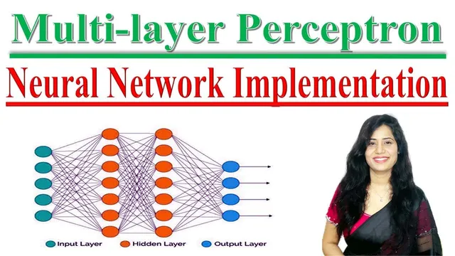
Multilayer perceptron (MLP) neural networks are a foundational feedforward model built to learn nonlinear patterns for prediction tasks like classification and regression. At the core, an MLP stacks layers of interconnected neurons: an input layer receives features, one or more hidden layers transform those features through weighted sums and nonlinear activation functions, and an output layer produces final predictions. Each connection carries a trainable weight, each neuron includes a trainable bias, and the activation function is what gives the network the ability to model complex, nonlinear relationships rather than only linear ones.
Training an MLP hinges on two complementary steps. Forward propagation pushes input data through the network layer by layer, computing outputs using the current weights, biases, and activation functions. A loss function then measures how far the network’s output is from the desired target, turning prediction error into a numeric signal. Backpropagation uses that error signal to adjust weights (and biases) to reduce the loss over time, with the practical goal of improving prediction accuracy.
Common activation functions mentioned include sigmoid, tanh, and ReLU, each used to introduce nonlinearity. For learning, the transcript highlights the standard pipeline: forward propagation to generate predictions, loss computation to quantify error, and backpropagation to minimize that error by updating parameters. The model’s applicability spans multiple domains: email spam detection (classification), image classification, weather or temperature forecasting (regression), and natural language processing tasks such as sentiment analysis or categorizing text into positive/negative labels.
The implementation portion demonstrates a binary classification MLP using TensorFlow in Google Colab. The workflow starts by installing TensorFlow, importing required libraries, and loading a dataset from Kaggle stored as two files—one documentation file and one CSV. The CSV includes feature columns (11 input features) and a binary target variable labeled Target, where 0 indicates no heart disease and 1 indicates heart disease. After inspecting the data distribution, the dataset is split into inputs (X) and labels (y), then divided into training and test sets using a 20% test size, a fixed random state, and stratification to preserve class balance.
Before training, the features are scaled using a preprocessing step (fit/transform on training and apply to test) so the network trains more reliably. The MLP architecture is then defined with 11 input features, a single hidden layer with 16 nodes using ReLU activation, and an output layer using sigmoid activation—appropriate for binary classification. Training uses binary cross-entropy as the loss function and accuracy as the metric, running for 100 epochs with a 20% validation split. The reported result is about 80.87% accuracy, followed by generating predictions on the test set and comparing predicted versus actual classes. The overall takeaway is a complete, lightweight template for building and training an MLP on a tabular binary dataset, adaptable to other case studies by swapping data, features, and network hyperparameters.
Cornell Notes
An MLP is a feedforward neural network that learns nonlinear relationships by stacking layers of neurons. Each neuron computes a weighted sum of inputs plus a bias, then applies a nonlinear activation function (commonly sigmoid, tanh, or ReLU). Training uses forward propagation to produce predictions, a loss function to measure error, and backpropagation to adjust weights to reduce that error. For binary classification, the output layer typically uses sigmoid activation and training often uses binary cross-entropy loss. A TensorFlow implementation in Colab demonstrates this pipeline on a Kaggle heart-disease dataset with 11 features, achieving about 80.87% accuracy after 100 epochs.
What makes an MLP different from a single-layer perceptron?
How do weights, biases, and activation functions work together in an MLP neuron?
Why do forward propagation, loss functions, and backpropagation form the training loop?
What activation and loss choices fit a binary classification MLP?
How was the dataset prepared before training in the implementation?
What MLP architecture and training settings were used, and what result was reported?
Review Questions
- How would changing the activation function in the hidden layer (e.g., ReLU to sigmoid) likely affect an MLP’s ability to learn and train stability?
- Why does stratifying the train/test split matter for binary classification datasets with imbalanced classes?
- If the loss decreases but accuracy stalls, what parts of the MLP setup (scaling, architecture, learning rate/optimizer, epochs) would you inspect first?
Key Points
- 1
An MLP learns nonlinear patterns by combining weighted sums, trainable biases, and nonlinear activation functions across input, hidden, and output layers.
- 2
Forward propagation generates predictions; a loss function quantifies error; backpropagation updates weights to reduce that error over time.
- 3
Sigmoid, tanh, and ReLU are common activation functions used to introduce nonlinearity into MLPs.
- 4
Binary classification typically pairs a sigmoid output layer with binary cross-entropy loss and evaluates performance using accuracy.
- 5
A practical workflow for tabular data includes splitting X/y, stratified train/test splitting, and feature scaling before training.
- 6
A simple TensorFlow MLP template can be adapted by changing dataset features, hidden-layer size, activation functions, and training hyperparameters like epochs and validation split.